Why air rises: lift on the large scale
- Read first
- Vorticity, The jet stream, CAPE, CIN and instability
A thunderstorm updraft can climb tens of meters per second. The rising air that covers a whole weather system moves a few centimeters per second, slower than a person walks, and it is still what makes the clouds and rain of a winter storm, and what cools and weakens the cap before a severe weather outbreak. This lesson measures that slow ascent, shows the continuity of mass that ties it to divergence aloft and convergence below, and works through its causes: jet streaks, warm air advection, the quasi-geostrophic omega equation in its traditional and Trenberth forms, Q vectors and isentropic lift. It ends with one storm, the record Midwest cyclone of October 26, 2010, computed from reanalysis data and checked against the rain and snow that fell.
- How slow large-scale ascent is, in centimeters per second and in omega, and why hours of it can cool a layer by several degrees and cut a cap's inhibition.
- Continuity: divergence aloft over convergence below, the level of nondivergence between them, and Dines compensation, computed from gridded winds.
- Jet streaks and temperature advection: the four-quadrant model, and warm and cold air advection read from an 850 hPa map.
- The omega equation in its traditional and Trenberth forms, each term in words, and the terms computed for a real storm.
- Q vectors, isentropic lift and frontal circulations, briefly.
- One storm put together: vorticity, the jet, temperature advection and the observed precipitation lining up.
How slow large-scale ascent is
Nobody measures the rising motion of a weather system directly. Holton's textbook, after listing the scales of midlatitude systems (horizontal wind about 10 m/s, length about 1,000 km), sets the vertical velocity scale at "W ∼1 cm s⁻¹" and notes that "the synoptic scale vertical velocity is not a directly measurable quantity"; it has to be deduced from the horizontal wind or the temperature field.[2] The synoptic scale is, in the AMS definition, the scale of weather systems "ranging in size from several hundred kilometers to several thousand kilometers, the scale of migratory high and low pressure systems."[1]
On weather maps the vertical motion is usually given as omega, ω, the vertical velocity in pressure coordinates, which the AMS writes as "ω = Dp/Dt": the rate at which the pressure around a moving parcel of air changes.[1] Rising air moves toward lower pressure, so ascent has negative omega. For large-scale motion Holton shows that omega and the ordinary vertical velocity w are tied by the hydrostatic equation:
ω ≈ −ρgw
where ρ is the air density and g gravity. He finds the other contributions to omega, the local pressure change and the ageostrophic wind blowing across isobars, about 10 and 1 hPa per day against "gρw ∼100 hPa d⁻¹", which is why "it is quite a good approximation."[2] Omega comes in pascals per second or microbars per second (1 µb/s = 0.1 Pa/s), sometimes in hectopascals per hour. At 700 hPa and 0 °C the density is 0.89 kg/m³, so −1 Pa/s is 11.4 cm/s of rise; at 850 hPa, about 10 cm/s; at 500 hPa and −20 °C, about 15 cm/s. Computed here.
| Rising air | Speed | Omega | Source |
|---|---|---|---|
| Synoptic-scale vertical velocity scale | about 1 cm/s | about −0.1 Pa/s (−100 hPa/day) | Holton [2] |
| Typical ascent ahead of a trough, this lesson's worked number | 2.4 cm/s at 700 hPa | −0.2 Pa/s (−2 µb/s) | Computed here |
| Strongest 700 hPa ascent in the October 26, 2010 cyclone | about 8 cm/s | −0.72 Pa/s | Reanalysis, computed here [12] |
| Frontal zones | about 10 cm/s | about −1 Pa/s | Holton [2] |
| Thunderstorm updraft, Sterling, VA, June 29, 2012 | about 50 m/s (half of 104) | hundreds of Pa/s | CAPE lesson |
The last row comes from the lesson on CAPE, CIN and instability, where 5,458 J/kg of CAPE sets a ceiling of 104 m/s and real updrafts reach about half. A thunderstorm updraft is a thousand times faster than the air rising under an upper trough. At 2 cm/s air climbs about 70 m an hour, 430 m in six hours; the updraft covers the same height in ten seconds. Doswell (1987) summed up the division of labor: "convective systems depend primarily on large-scale processes for developing a suitable thermodynamic structure, while mesoscale processes act mainly to initiate convection."[9]
Why slow ascent matters
Rising air expands and cools, as the lesson on air parcels and adiabatic cooling explains, at the dry adiabatic rate of 9.8 °C per kilometer until it saturates. Slow ascent works on a whole layer at once and keeps working for hours. At a fixed level the temperature changes by what the wind carries in and by what the vertical motion does to the layer. Holton's adiabatic method writes this as:[2]
∂T/∂t = −V·∇T + Sp ω
where Sp = −(T/θ) ∂θ/∂p is the static stability, positive when potential temperature θ increases upward. The first term is horizontal advection. The second says that rising air (ω < 0) cools the level, and cools it fastest where the layer is most stable, because there the air brought up from below had the lowest potential temperature to begin with. A cap is the most stable layer in the sounding, so ascent works on it hardest. The lesson on inversions and the cap introduces the cap; this is the mechanism that can cool it from above.
A worked number, on the capped morning that lesson examines: Norman, Oklahoma, 7 am CDT April 22, 2001. Between 800 and 700 hPa the sounding's potential temperature rises so steeply that Sp is 0.099 K per hPa. With ω = −0.2 Pa/s, that layer cools at 0.2 × 0.00099 K per second, 4.3 °C in six hours, without any cold air being carried in. Computed here from the Iowa Environmental Mesonet's archive of the sounding.[19]
- Temperature, 7 am CDT
- Dew point, 7 am
- After 6 hours of ascent, computed
- Temperature observed at 1 pm
- CIN, 7 am surface parcel
Table: the 7 am sounding lifted for six hours, surface parcel held at 7 am values
| Omega in the free troposphere | Air ending at 700 hPa rose, hPa | Change at 750 hPa, °C | Change at 700 hPa, °C | Surface parcel CIN, J/kg | Surface parcel CAPE, J/kg |
|---|---|---|---|---|---|
| Observed 7 am sounding | 0 | 0.0 | 0.0 | −607 | 11 |
| −0.10 Pa/s (−1.0 µb/s, 1.2 cm/s at 700 hPa) | 22 | −4.8 | −0.2 | −477 | 180 |
| −0.20 Pa/s (−2.0 µb/s, 2.4 cm/s at 700 hPa) | 43 | −7.9 | −0.8 | −369 | 275 |
| −0.30 Pa/s (−3.0 µb/s, 3.6 cm/s at 700 hPa) | 65 | −8.7 | −5.5 | −271 | 350 |
| −0.50 Pa/s (−5.0 µb/s, 6.0 cm/s at 700 hPa) | 108 | −9.6 | −9.9 | −130 | 442 |
The figure does the full calculation: each level of the 7 am sounding is traced back to where it would have started six hours earlier, then lifted dry-adiabatically, or along the saturated adiabat if it reaches saturation. The table under the figure repeats it for other values of omega. At −0.1 Pa/s the CIN falls to −477 J/kg; at −0.3, to −271; at −0.5 Pa/s, 6 cm/s, to −130. The whole inversion rises and cools, which is why the change at a fixed level such as 700 hPa can be small while the layer below it cools by 8 °C: the air now at 700 hPa came from the warmest part of the cap.
On the real day the cap weakened faster than ascent alone explains. The observed 1 pm sounding had −70 J/kg of CIN, with the ground also heated from 18 to 22 °C, and the study of the day quoted in the cap lesson found that "horizontal advection was the primary agent of cooling within the CIN layer" in its model.[18] The calculation here isolates one term: six hours of large-scale ascent between −0.1 and −0.5 Pa/s takes a fifth to four fifths of the inhibition out of a strong cap, and it cools the whole layer, which heating at the ground does not. Continued long enough, the same ascent brings a layer to saturation, which is how the broad cloud shields of winter storms form without any buoyant updraft at all.
Continuity: divergence and convergence
Air that rises has to be replaced from the sides below and has to go somewhere above. The divergence measures the spreading. The AMS defines it as "the expansion or spreading out of a vector field; also, a precise measure thereof," and notes that in meteorology it "usually refers to the two-dimensional horizontal divergence of the velocity field," ∂u/∂x + ∂v/∂y. Convergence is "negative divergence."[1] The mass budget is the continuity equation, which in pressure coordinates the AMS writes as:[1]
∇p·V + ∂ω/∂p = 0
Horizontal divergence on a pressure surface is matched by a change of omega with pressure. Where the air converges near the ground, omega must become more negative going up: the air rises out of the converging layer. Where it diverges aloft, omega returns toward zero: the rising air spreads out and stops. The AMS gives the sizes: "The geostrophic wind has divergence of the order of 10⁻⁶ s⁻¹; the wind field associated with migratory cyclonic systems, 10⁻⁵ s⁻¹; motions of smaller scale (such as gravity waves, frontal waves, and cumulus convection) have characteristic divergence one or two orders of magnitude greater."[1]
Divergence is hard to measure because it is small compared with the winds that produce it. Holton warns that "a 10% error in evaluating one of the wind components ... can easily cause the estimated divergence to be in error by 100%," and for that reason does not recommend the continuity method for estimating vertical motion from observed winds.[2] A reanalysis helps, because its winds have been made consistent with each other and with a model's physics. The maps below are computed from the NCEP/NCAR Reanalysis 1 on its 2.5 degree grid, at 12 UTC (7 am CDT) October 26, 2010, as the storm deepened over Minnesota.[12]
Table: divergence (×10⁻⁵ s⁻¹) and 500 hPa omega (Pa/s) at reanalysis grid points, 12 UTC October 26, 2010
| Grid point nearest | 300 hPa divergence | 850 hPa divergence | 500 hPa omega |
|---|---|---|---|
| Bismarck, ND area | 0.75 | −1.68 | −0.21 |
| Minneapolis, MN area | 1.52 | −1.69 | −0.35 |
| Duluth, MN area | 1.74 | −1.56 | −0.51 |
| Des Moines, IA area | 0.67 | −1.27 | −0.16 |
| Chicago, IL area | 1.04 | −0.74 | −0.38 |
| Detroit, MI area | 1.07 | −0.57 | −0.12 |
| Kansas City, MO area | −0.16 | 0.23 | 0.18 |
| St. Louis, MO area | −0.27 | −1.01 | −0.42 |
| Nashville, TN area | −0.36 | −0.92 | −0.29 |
| Dallas, TX area | 0.17 | −0.33 | 0.03 |
Dines compensation and the level of nondivergence
The two maps are nearly mirror images, and that is not a coincidence. The AMS calls it Dines compensation: the "property whereby the sign of the horizontal divergence reverses at least once in the troposphere or the stratosphere. This implies that the vertically integrated divergence and the associated surface pressure tendency are small residuals of much larger contributions."[1] Holton puts it the same way: "there is a strong tendency for vertical compensation. Thus, when there is convergence in the lower troposphere there is divergence aloft, and vice versa."[2] Between the two layers lies the level of nondivergence, which the AMS describes as the "midtropospheric surface that separates the major regions of horizontal convergence and divergence," "usually assumed to be in the vicinity of 500 mb."[1]
Table: area averages over the dashed box, 12 UTC October 26, 2010, NCEP/NCAR Reanalysis
| Pressure, hPa | Divergence, ×10⁻⁵ s⁻¹ | Omega, Pa/s | Grid points |
|---|---|---|---|
| 925 | −1.86 | −0.06 | 13 |
| 850 | −0.83 | −0.17 | 18 |
| 700 | −0.62 | −0.25 | 18 |
| 600 | −0.53 | −0.31 | 18 |
| 500 | −0.36 | −0.35 | 18 |
| 400 | 0.34 | −0.36 | 18 |
| 300 | 1.41 | −0.28 | 18 |
| 250 | 2.22 | −0.18 | 18 |
| 200 | 1.92 | −0.08 | 18 |
| 150 | 0.74 | −0.01 | 18 |
| 100 | −0.16 | 0.01 | 18 |
The profile can be checked against the continuity equation. Integrated from the bottom, omega at a level is its value lower down minus the integral of divergence over pressure. From 925 hPa, where the box average is −0.06 Pa/s, to 500 hPa the average convergence is about 0.7 ×10⁻⁵ s⁻¹ over 425 hPa: 0.73 ×10⁻⁵ s⁻¹ × 42,500 Pa is 0.31 Pa/s, so omega at 500 hPa should be about −0.37 Pa/s. The reanalysis gives −0.36. The ascent is fastest at the level of nondivergence because that is where the converging air below stops feeding it and the diverging air above starts draining it.
Integrated through the whole column, the convergence below and the divergence above almost cancel. Here the residual is net divergence worth 0.05 Pa/s, a sixth of the convergence in the lower half. By Holton's surface pressure tendency equation, net divergence over a column lowers the pressure at the ground; this residual would be 1.8 hPa an hour, the right order for a storm that deepened from a 1000 hPa height of −138 m to −329 m between 00 and 18 UTC. Holton adds the caution that the net "is then a small residual in the vertical integral of a poorly determined quantity," so the number is an illustration, not a forecast.[2][12] Uccellini and Kocin state the rule that follows for storms: "A net reduction in mass is required for surface cyclones to develop, whereby upper-tropospheric mass divergence exceeds low-level convergence."[6]
Jet streaks
One source of divergence aloft is the jet streak. The jet stream lesson introduces it; the AMS entry calls the jet streak "the region of a jet stream axis with the greatest winds."[1] Air entering a streak speeds up and air leaving it slows down, and in neither case is the wind in geostrophic balance. The difference, the ageostrophic wind, blows across the jet and piles air up on one side and removes it from the other. Uccellini and Kocin (1987) described the textbook pattern: the entrance region "is marked by a transverse ageostrophic component directed toward the cyclonic-shear side of the jet," the upper branch of "a direct transverse circulation" with "rising (sinking) motion on the anticyclonic or warm (cyclonic or cold) side of the jet"; in the exit region the ageostrophic wind points the other way, and the circulation is indirect, with "rising (sinking) motion on the cyclonic or cold (anticyclonic or warm) side of the jet."[6]
| Quadrant (Northern Hemisphere, facing downstream) | Upper-level flow | Vertical motion below |
|---|---|---|
| Right entrance (warm side, upstream) | Divergence | Rising |
| Left entrance (cold side, upstream) | Convergence | Sinking |
| Left exit (cold side, downstream) | Divergence | Rising |
| Right exit (warm side, downstream) | Convergence | Sinking |
The four quadrants of a straight jet streak, from Uccellini and Kocin's Figure 3 (after Bjerknes, 1951).[6] Durran and Snellman (1987) explain the exit circulation with the balance argument of the next sections. In their example the westerly wind blows out of a region of high speed into one of low speed, so the geostrophic wind "will advect itself in a manner which increases the wind speed throughout the entire region" while the temperature pattern stays put, leaving a wind shear "too strong to be in thermal wind balance." The ageostrophic circulation corrects it: "the northerly wind in the upper branch of the ageostrophic circulation decelerates the upper-level westerlies while the southerly wind on the lower branch accelerates the lower-level westerlies," and its rising branch is on the cold side.[5] Uccellini and Kocin add the caveat that matters on real maps: curvature can mask the pattern, and "although the transverse circulations are normally depicted on a two-dimensional vertical plane, the existence of indirect and direct circulations is a consequence of three-dimensional variations in the ageostrophic winds and upper-level divergence that cannot be fully described in terms of simple two-dimensional, straight-line jet streak dynamics."[6]
- Wind speed, m/s (40, 50, 60, 70)
- Arrows: wind at 250 hPa, 20 m/s and faster
Table: 250 hPa wind speed (m/s) and divergence (×10⁻⁵ s⁻¹), 00 UTC October 26, 2010
| Grid point nearest | Wind speed | Divergence |
|---|---|---|
| Left entrance (average over a 7.5° by 10° box) | −0.69 | |
| Right entrance (average over a 7.5° by 10° box) | −0.24 | |
| Left exit (average over a 7.5° by 10° box) | 0.38 | |
| Right exit (average over a 7.5° by 10° box) | −1.15 | |
| Bismarck, ND area | 34.4 | 1.83 |
| Minneapolis, MN area | 34.6 | 2.47 |
| Duluth, MN area | 32.5 | 1.27 |
| Des Moines, IA area | 41.0 | 2.71 |
| Chicago, IL area | 34.6 | 0.01 |
| Detroit, MI area | 28.3 | −0.68 |
| Kansas City, MO area | 49.3 | 3.30 |
| St. Louis, MO area | 35.0 | −0.11 |
| Nashville, TN area | 22.3 | −0.56 |
| Dallas, TX area | 29.2 | 1.34 |
| Denver, CO area | 36.9 | −1.48 |
| Salt Lake City, UT area | 75.2 | −2.04 |
That is the usual experience: the four-quadrant model describes a straight streak, and real streaks bend through troughs and ridges, where the divergence of curved flow is added to it. The trough lesson describes the divergence downstream of a trough axis, and the vorticity lesson ties both to vorticity advection. The omega equation below combines them.
Warm and cold air advection
Warm air advection is the wind carrying warmer air into a place; cold air advection, colder. The AMS defines advection as "the process of transport of an atmospheric property solely by the mass motion (velocity field) of the atmosphere; also, the rate of change of the value of the advected property at a given point," and notes that "often, particularly in synoptic meteorology, advection refers only to the horizontal or isobaric components of motion, that is, the wind field as shown on a synoptic chart."[1] For temperature:
Temperature advection = −V·∇T = −(u ∂T/∂x + v ∂T/∂y)
It is the wind speed times the temperature gradient times the cosine of the angle between the wind and the gradient: largest where strong wind blows straight across tightly packed isotherms, zero where the wind runs along them. A 20 m/s wind blowing straight across isotherms spaced 1 °C per 100 km warms or cools the air at a point by 20 × 0.00001 °C per second, 17 °C per day. On an 850 hPa chart, the reading rule follows: look for wind barbs crossing the isotherms. Wind blowing from warm toward cold is warm air advection; from cold toward warm, cold air advection. Near the ground friction turns the wind across the isobars, as the wind lesson shows; at 850 hPa, about 1.5 km up, the wind is closer to geostrophic and the pattern is cleaner.
- Isotherms every 5 °C
- Arrows: wind at 850 hPa
Table: 850 hPa temperature (°C), wind speed (m/s) and temperature advection (°C per day), 00 UTC October 26, 2010
| Grid point nearest | Temperature | Wind speed | Advection |
|---|---|---|---|
| Bismarck, ND area | 5.8 | 9.5 | −3.7 |
| Minneapolis, MN area | 11.9 | 15.9 | 15.2 |
| Duluth, MN area | 8.5 | 14.5 | 13.2 |
| Des Moines, IA area | 14.6 | 20.2 | 11.9 |
| Chicago, IL area | 14.4 | 14.3 | 8.9 |
| Detroit, MI area | 10.6 | 11.4 | 6.6 |
| Kansas City, MO area | 14.9 | 19.7 | 7.4 |
| St. Louis, MO area | 15.9 | 26.7 | 3.4 |
| Nashville, TN area | 15.4 | 19.9 | 7.0 |
| Dallas, TX area | 22.0 | 20.3 | 21.7 |
| Denver, CO area | below ground | ||
| Salt Lake City, UT area | below ground |
Warm advection alone does not make air rise, and the air at a point does not warm by the full advection rate. On this map the ascent is strongest along a band from Kansas City to Minnesota, where 700 hPa omega reached −0.69 Pa/s. Why rising air goes with warm advection, and why the relationship is looser than the maps suggest, is the subject of the next three sections.
Why balance demands vertical motion
The large-scale atmosphere stays close to two balances: the hydrostatic balance between pressure and weight, covered in the air pressure lesson, and the geostrophic balance between the pressure gradient and the Coriolis force, covered in the wind lesson. Together they tie the change of the wind with height to the horizontal temperature gradient: the thermal wind. The wind, advecting temperature and vorticity, constantly works to break that tie. Durran and Snellman (1987) state the result: "The quasi-geostrophic vertical velocity (and ageostrophic horizontal winds) are those motions which are required to keep the geostrophic advection from producing large disruptions in the hydrostatic and geostrophic balances."[5]
Holton's example makes it concrete. Over a surface low, positive vorticity advection aloft makes the 500 hPa vorticity increase, which requires the 500 hPa heights to fall, which requires the layer below to cool. With little horizontal temperature advection over the low, "the only way to cool the atmosphere as required by the thickness tendency is by adiabatic cooling through the vertical motion field." His summary: "the vertical motion field is just that required to ensure that changes in vorticity will be geostrophic and changes in temperature will be hydrostatic."[2] This is quasi-geostrophic theory, which the AMS calls "relatively accurate for synoptic-scale atmospheric motions" but unable to "accurately describe some atmospheric structures such as fronts or small strong low pressure cells."[1]
The omega equation
Combining the quasi-geostrophic vorticity and thermodynamic equations to eliminate the height tendency gives the omega equation, which the AMS describes as "a diagnostic equation by which the vertical velocity in pressure coordinates ... may be calculated according to quasigeostrophic theory."[1] In Holton's traditional form, for flow without heating:[2]
(∇² + (f0²/σ) ∂²/∂p²) ω = (f0/σ) ∂/∂p [Vg·∇(ζg + f)] + (1/σ) ∇²[Vg·∇(−∂Φ/∂p)]
Vg is the geostrophic wind, ζg its vorticity and f the Coriolis parameter (f0 a constant value of it), Φ the geopotential, whose derivative −∂Φ/∂p is proportional to temperature (it equals RT/p), and σ a static stability. Three pieces, in words:
- The left side: omega, upside down
- The operator is a three-dimensional Laplacian. Holton shows that for a wave-like pattern it is proportional to −ω, so "upward motion is forced where the right-hand side ... is positive and downward motion is forced where it is negative." The COMET Program's omega equation lab puts it the same way: "the LHS differential operator behaves qualitatively like a negative sign."[2][8] The Laplacian also smooths: the response to a small, sharp forcing is weaker and broader than the forcing itself.
- First term: differential vorticity advection
- The change with height of the advection of absolute vorticity. Where cyclonic vorticity advection increases with height (typically: strong at 500 hPa between a trough and the ridge downstream, weak near the ground), the term forces ascent. Galarneau's guide for the National Severe Storms Laboratory: "For the example of a 500 hPa trough located upstream of the attendant surface cyclone, term A is > 0 downstream of the 500 hPa trough and over the surface cyclone resulting in forcing for ascent over the surface cyclone."[7] The vorticity lesson shows how to read vorticity advection on a 500 hPa map.
- Second term: the Laplacian of temperature advection
- Proportional to the horizontal Laplacian of the temperature advection. A Laplacian is largest, with the sign here, where the quantity has a local maximum, so the term forces ascent at a maximum of warm air advection and descent at a maximum of cold air advection, not simply wherever there is warm advection. Trenberth: "upward motion occurs in regions of pronounced warm advection (where warm advection is a maximum)."[3]
- 500 hPa height contours
- Isotherms
- Forced ascent
- Forced descent
The equation is diagnostic: it gives omega from the height field at one moment, with no time derivative. Holton notes that "direct wind observations are not required at all," but that its terms "employ higher order derivatives" that are hard to estimate "from noisy observational data."[2] It also leaves out heating: latent heat released in cloud strengthens the ascent that produced it, which is one reason a real storm's rising motion is often stronger and narrower than its quasi-geostrophic forcing.
The Trenberth form
The two traditional terms look like separate processes, but they are not independent. Trenberth (1978) wrote: "The problem with this interpretation is in the separation into these two terms, since they are not usually independent because each contains a common cancelling component." He showed that "for the middle troposphere ... both terms contribute nearly equal amounts to the vertical motion and part of each term cancels."[3] Holton adds that the two terms "are not invariant under a Galilean transformation": adding a uniform wind to the whole pattern changes each term "without changing the net forcing."[2]
Expanding the terms, dropping the cancelling pieces and one that is small in the middle troposphere, Trenberth arrived at a single term:
(∇² + (f0²/σ) ∂²/∂p²) ω ≈ (2f0/σ) (∂Vg/∂p)·∇(ζg + f)
∂Vg/∂p is the thermal wind (with a sign: it points opposite to the increase of wind with height), which blows along the isotherms with cold air to its left. In Trenberth's words, the result is "very useful for estimating areas of upward or downward motion visually from a chart containing geopotential height and thickness contours, since upward motion occurs where there is cyclonic advection of vorticity by the thermal wind."[3] On a chart of 500 hPa vorticity and 1000 to 500 hPa thickness, follow the thickness lines with the cold air on the left; where vorticity decreases in that direction, air rises. He cautioned that the approximation "is fairly crude" and fits best in the middle troposphere, "600 and 400 mb," being "less accurate below 700 mb or above 350 mb."[3] Durran and Snellman recommended it for the forecaster working by eye: "the easiest and most accurate approach is to examine the advection of vorticity by the thermal wind as suggested by Trenberth (1978) and Sutcliffe (1947)."[5]
Holton's text writes the same approximation without Trenberth's factor of two; the pattern, which is what a forecaster reads, is the same.[2]
The terms computed
The terms can be computed from gridded heights and temperatures. The figure does it for 12 UTC October 26, 2010, near 700 hPa, with the geostrophic wind from the reanalysis heights, vorticity advection at 850 and 500 hPa, and temperature advection at 700 hPa, and compares each forcing with the reanalysis's own 700 hPa ascent. As in the studies it follows, it shows the forcing, not a solved omega; by the left-hand side's "negative sign," forcing for rising should sit over rising air.
- Reanalysis rising motion at 700 hPa, 0.2 and 0.4 Pa/s
Table: forcing terms near 700 hPa (×10⁻¹² Pa m⁻² s⁻¹) and reanalysis omega, 12 UTC October 26, 2010. Pattern correlation with the reanalysis ascent: vorticity term 0.58, warm advection term 0.02, sum 0.56, Trenberth 0.3, Q-vector 0.53
| Grid point nearest | Vorticity term | Warm advection term | Sum | Trenberth | Q-vector | 700 hPa omega, Pa/s |
|---|---|---|---|---|---|---|
| Bismarck, ND area | −0.3 | 1.4 | 1.1 | 3.0 | 2.2 | −0.16 |
| Minneapolis, MN area | 5.1 | −3.5 | 1.6 | −0.3 | 0.3 | −0.41 |
| Duluth, MN area | 3.6 | 0.5 | 4.1 | 3.4 | 2.8 | −0.44 |
| Des Moines, IA area | 5.0 | −9.0 | −3.9 | −7.3 | −4.9 | −0.18 |
| Chicago, IL area | 3.5 | −2.0 | 1.4 | −2.1 | 2.1 | −0.23 |
| Detroit, MI area | −1.7 | 4.2 | 2.5 | 1.0 | 2.1 | 0.07 |
| Kansas City, MO area | −0.6 | −4.6 | −5.2 | −9.6 | −6.0 | 0.27 |
| St. Louis, MO area | 4.1 | −6.2 | −2.2 | −7.7 | −2.3 | −0.28 |
| Nashville, TN area | 1.0 | 0.6 | 1.6 | −1.0 | 1.8 | −0.43 |
| Dallas, TX area | 1.1 | 1.0 | 2.1 | 2.1 | 2.5 | −0.02 |
| Denver, CO area | 0.23 | |||||
| Salt Lake City, UT area | −0.03 |
Three lessons come out of the maps. The temperature term alone says almost nothing about where the air was rising on this morning, even though the storm was full of warm and cold advection; its pattern is a ring of opposite signs that the vorticity term largely offsets, Trenberth's cancellation in action. The sum and the Q-vector form, which should agree in theory, agree in practice (0.56 and 0.53). And Trenberth's single term does worse here (0.30), as he warned it would below 700 hPa and in a mature system: this storm was occluding, the situation in which, he noted, Krishnamurti "found that total vertical motion was largely a thermal contribution."[3] None of the forcing patterns is the omega itself, which also depends on the latent heat released in the clouds; the reanalysis ascent includes it.
Q vectors
Hoskins, Draghici and Davies (1978) rewrote the forcing so that the cancellation never appears. As summarized by Sanders and Hoskins (1990), "the right-hand side of the omega equation ... could be written in a way that avoids this potential cancellation effect":[4]
(σ∇² + f0² ∂²/∂p²) ω = −2∇·Q
"This compact form of the equation shows that the vertical motion tends to be upward when the field of Q-vectors is convergent." The Q vector is the rate at which the geostrophic wind changes the horizontal temperature gradient. Sanders and Hoskins gave a way to estimate it from a map: travel "along the isotherm with the cold air to the left," note "the vector change of the geostrophic wind," and rotate it 90° clockwise; "its magnitude is proportional to the magnitude of the vector rate of change multiplied by the strength of the temperature gradient."[4] Galarneau's guide lists the advantages over the traditional form: the forcing uses a single pressure level, is Galilean invariant, has "no cancellation problem between forcing terms" and neglects no term.[7] Durran and Snellman concluded that "the Q-vector approach appears to provide the best means of calculating vertical motions numerically."[5]
Isentropic lift
A different way to see the same ascent is to follow the air on a surface of constant potential temperature, an isentropic surface, "a surface in space on which entropy (or, in meteorology, potential temperature) is everywhere equal."[1] Air that neither gains nor loses heat stays on its surface. Isentropic surfaces slope upward toward the cold air, so air flowing on one toward colder latitudes has to climb. The National Weather Service defines isentropic lift as the "lifting of air that is traveling along an upward-sloping isentropic surface," adding that it "often is referred to erroneously as overrunning" and that it is often "characterized by widespread stratiform clouds and precipitation, but may include elevated convection in the form of embedded thunderstorms."[10]
An isentropic chart shows pressure on the surface, so the reading rule is simple. Scott Truett of the Des Moines forecast office wrote in 1987: "Winds blowing toward lower pressure would tend to be rising," with a caveat: "The isentropic surfaces themselves are moving," though "typically the movement of the isentropic surface is slower than the wind," and "if the isobars are tightly packed and winds are strong across the isobars, the lift is rapid and intense."[11] In symbols, following the air on its surface:
ω = (∂p/∂t)θ + V·∇θp
The second term is the upglide, the wind blowing across the isobars of the surface; the first is the motion of the surface itself. Durran and Snellman: "The vertical motion at a point on an isentropic chart is proportional to the wind speed relative to the motion of the isentropic surface times the isentropic pressure-gradient in the direction of the relative wind vector."[5] A worked number from the figure: at 00 UTC October 26, 2010, the 310 K surface lay at 655 hPa near Kansas City and 612 hPa near Des Moines, 280 km north. A south wind of 16 to 24 m/s blowing up that slope, 0.15 hPa per km, gives about 0.3 Pa/s of ascent; the reanalysis computed here gives −0.35 Pa/s of upglide at Des Moines and −0.57 Pa/s of omega at 700 and 500 hPa.
- Pressure on the 310 K surface, hPa
- Arrows: wind on the surface
Table: the 310 K surface at 00 UTC October 26, 2010: pressure (hPa), wind speed (m/s), omega from upglide alone and with the surface’s motion (Pa/s), and the reanalysis 700 hPa omega
| Grid point nearest | Pressure | Wind speed | Upglide omega | Isentropic omega | Reanalysis omega, 700 hPa |
|---|---|---|---|---|---|
| Bismarck, ND area | 528 | 6.5 | 0.10 | −0.06 | −0.15 |
| Minneapolis, MN area | 584 | 21.0 | −0.11 | −0.10 | −0.33 |
| Duluth, MN area | 581 | 14.6 | −0.04 | 0.00 | −0.07 |
| Des Moines, IA area | 612 | 24.8 | −0.35 | −0.36 | −0.57 |
| Chicago, IL area | 608 | 16.7 | −0.17 | −0.05 | −0.01 |
| Detroit, MI area | 613 | 12.0 | 0.01 | 0.07 | 0.07 |
| Kansas City, MO area | 655 | 21.2 | −0.13 | −0.40 | −0.69 |
| St. Louis, MO area | 707 | 23.5 | −0.33 | −0.23 | −0.15 |
| Nashville, TN area | 699 | 23.0 | −0.39 | −0.21 | 0.10 |
| Dallas, TX area | 830 | 20.2 | −0.11 | ||
| Denver, CO area | 394 | 28.0 | 0.39 | 0.08 | 0.42 |
| Salt Lake City, UT area | 459 | 30.6 | 0.06 | 0.19 | 0.00 |
The two panels differ, and the difference is Truett's caveat in numbers. Near Omaha the wind blew slightly down the surface (+0.09 Pa/s of upglide), but the surface itself was rising so fast that the air on it rose at −0.38 Pa/s, close to the reanalysis's −0.47 at 700 hPa. Isentropic analysis is at its best where the flow is steady and the surface moves little: the classic case is the warm, moist air gliding up over a warm front, the stratiform rain shield that the NWS definition describes.
Frontal circulations
Fronts concentrate all of this into narrow zones. The AMS defines frontogenesis as "the initial formation of a front or frontal zone. In general, an increase in the horizontal gradient of an airmass property, principally density, and the development of the accompanying features of the wind field that typify a front."[1] As the flow squeezes the isotherms together, the thermal wind balance is disturbed again, and a circulation across the front restores it. Holton: "The secondary circulation associated with frontogenesis is required to maintain the thermal wind balance between the along-front flow and the cross-front temperature gradient in the presence of advective processes that tend to destroy this balance." In frontal zones "the vertical velocity scale is ∼10 cm s⁻¹," ten times the synoptic scale.[2]
Q vectors show the frontal circulation directly. The AMS: "The Q vector tends to point in the direction of rising air. If Q points toward warm air, the geostrophic flow is frontogenetic. If Q points toward cold air, the geostrophic flow is frontolytic."[1] Sanders and Hoskins drew the lesson that "the frontogenetical forcing, rather than the existence of a front, accounts for the frontal patterns of vertical motion and weather": a front that is being strengthened has warm air rising and cold air sinking; one that is being weakened can have the opposite, and little weather.[4] Fronts themselves, and the weather along each kind, are the subject of the weather fronts lesson in the next unit.
Putting it together: October 26, 2010
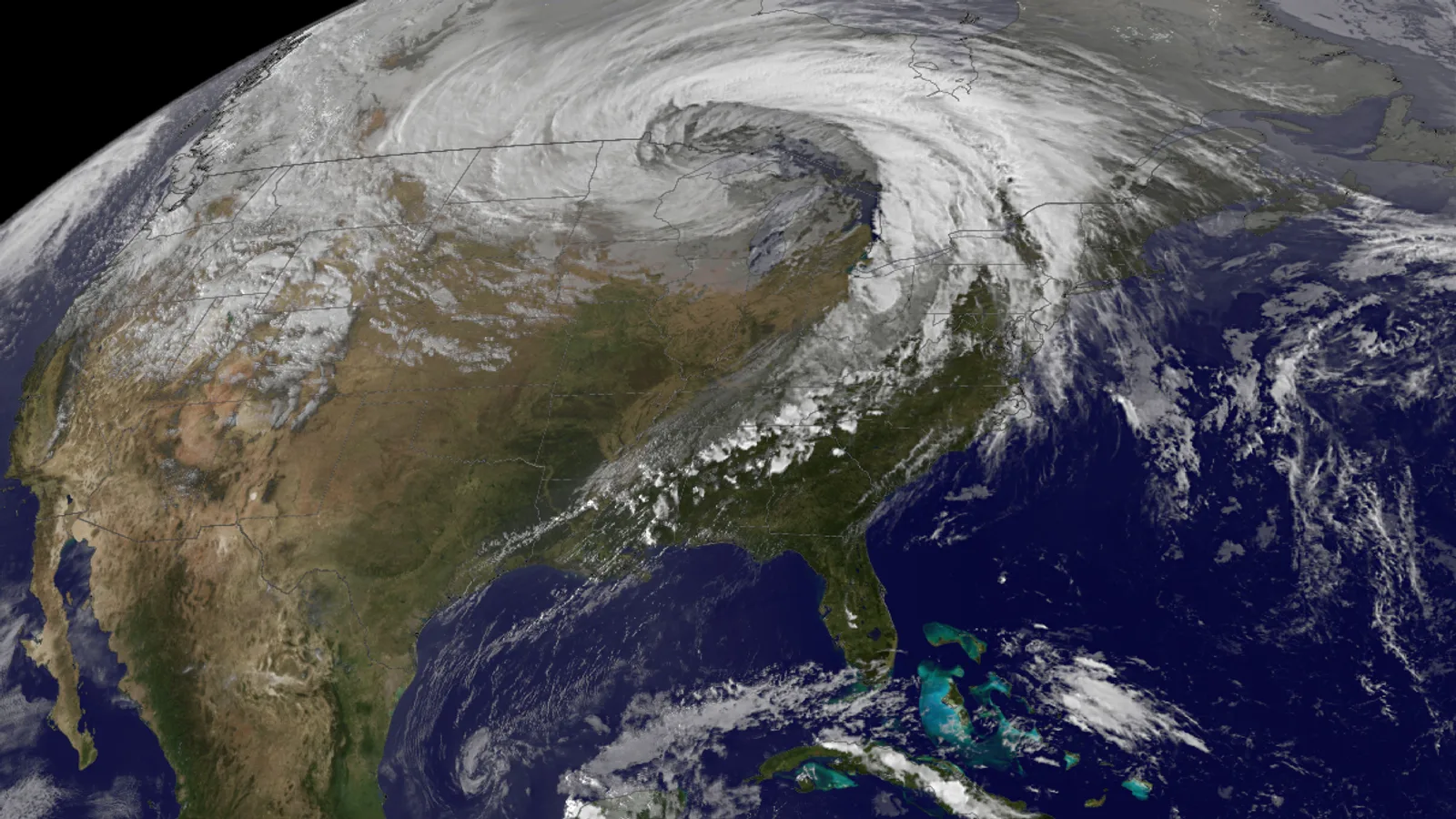
On October 26, 2010, a low crossed Minnesota and set records. The National Weather Service office in Milwaukee: "Bigfork, Minnesota recorded the lowest pressure in the U.S. for this particular storm. Bigfork had a minimum sea level pressure of 955.2 millibars (28.21") at 5:13 PM CDT." Superior, Wisconsin set that state's record, 961.3 millibars.[15] The air pressure lesson shows the barogram at International Falls, where the pressure fell 33.8 hPa in a day. The Storm Prediction Center logged 57 tornado reports and 339 damaging wind reports in the 24 hours from 7 am CDT on the 26th.[17] Every ingredient of this lesson was on the maps at 7 am.
- Vorticity above 14, 18 and 22 ×10⁻⁵ s⁻¹; wind 40, 50, 60 and 70 m/s and more; warm air advection
- Cold air advection
- Precipitation 1, 5, 10 and 25 mm and more
- Heights (a, b); mean ascent 0.2 and 0.3 Pa/s, dashed 0.1 (d)
Table: the four panels at reanalysis grid points: 500 hPa absolute vorticity (×10⁻⁵ s⁻¹), 300 hPa wind (m/s) and 850 hPa temperature advection (°C per day) at 12 UTC October 26, 2010; mean 700 hPa omega (Pa/s) and observed precipitation (mm, averaged over the 2.5-degree cell) for the 24 hours from 12 UTC October 26
| Grid point nearest | Vorticity | 300 hPa wind | Advection | Mean omega | Precipitation |
|---|---|---|---|---|---|
| Bismarck, ND area | 15.6 | 20.3 | −8.3 | −0.34 | 9.7 |
| Minneapolis, MN area | 19.9 | 33.7 | −4.4 | −0.16 | 15.3 |
| Duluth, MN area | 14.5 | 30.6 | 11.6 | −0.42 | 31.3 |
| Des Moines, IA area | 22.7 | 35.8 | −29.1 | 0.16 | 4.2 |
| Chicago, IL area | 12.6 | 42.0 | −14.0 | 0.09 | 6.0 |
| Detroit, MI area | 6.1 | 23.6 | 4.1 | 0.02 | 7.7 |
| Kansas City, MO area | 22.4 | 44.3 | −24.5 | 0.33 | 0.2 |
| St. Louis, MO area | 10.5 | 57.7 | −18.0 | −0.06 | 3.4 |
| Nashville, TN area | 4.0 | 32.7 | 3.1 | −0.32 | 19.3 |
| Dallas, TX area | 8.0 | 42.7 | −20.2 | −0.01 | 0.0 |
| Denver, CO area | 9.5 | 60.2 | below ground | 0.26 | 1.0 |
| Salt Lake City, UT area | 14.1 | 73.8 | below ground | 0.02 | 3.2 |
A forecaster's order of reading, applied to the four panels:
- 500 hPa vorticity. The vorticity maximum over Iowa, with the flow carrying it north and east, puts cyclonic vorticity advection over Wisconsin, Minnesota and the western Great Lakes: the first term of the omega equation, forcing ascent there.
- 300 hPa jet. The jet enters the trough from the west. Downstream of the trough the flow spreads and slows, and the divergence map of the continuity section shows 2 to 3 ×10⁻⁵ s⁻¹ over the Great Lakes, over the region of ascent.
- 850 hPa advection. Warm air advection wraps around the north and east of the low, 17 °C per day over Lake Superior; cold air advection floods Missouri and southern Iowa behind the cold front. By the second term, ascent north and east of the low and sinking behind the front.
- Continuity. Under the divergence aloft, the 850 hPa air converges into the low, the level of nondivergence sits near 445 hPa, and the column loses mass: the low deepens.
- The outcome. Precipitation fell where the reanalysis air rose. Across the 135 grid cells with gauge data, the correlation between the 24-hour mean ascent and the observed precipitation is 0.68; where the mean ascent exceeded 0.2 Pa/s the cells averaged 19.7 mm, and where the air sank at more than 0.1 Pa/s, 0.5 mm.
The second band of ascent in panel (d), from the Ohio Valley to the Gulf Coast, runs along the cold front, where a narrow line of storms produced most of the day's wind and tornado reports. There the large-scale ascent set the stage, and the front and the storms' own updrafts did the lifting.
What the large scale does not do
Quasi-geostrophic reasoning explains the broad pattern and misses the details. Doswell's abstract states the boundary: "Large-scale processes are limited, by definition, to those which are quasi-geostrophic," and they matter mainly "for developing a suitable thermodynamic structure, while mesoscale processes act mainly to initiate convection."[9] The CAPE lesson's three ways to lift a parcel make the same point from the parcel's view: heating, boundaries and large-scale ascent, with the last working on the cap rather than lifting parcels to their level of free convection. Latent heating, friction, terrain and the fine structure of fronts and jets all fall outside the equation. The lesson on how tornadoes form picks up where this one stops.
Check yourself
-
A model shows −0.4 Pa/s at 700 hPa. About how fast is the air rising, and how far does it rise in 12 hours?
Answer
At 700 hPa −1 Pa/s is about 11 cm/s, so −0.4 Pa/s is about 4.5 cm/s. In 12 hours (43,200 s) that is about 2 km: 0.4 Pa/s is 14.4 hPa an hour, 173 hPa in all.
-
Why does ascent cool a stable layer at a fixed height more than it cools a nearly dry-adiabatic one?
Answer
The cooling at a fixed level is Spω: the air arriving from below has cooled adiabatically on the way, and in a stable layer it started with a much lower potential temperature than the air it replaces. In a dry-adiabatic layer potential temperature is the same at every level, so lifted air arrives at the same temperature as the air it replaces and nothing changes.
-
Convergence at 850 hPa is 2 ×10⁻⁵ s⁻¹ through a 150 hPa deep layer above the ground. What omega does continuity give at the top of the layer?
Answer
ω = −(convergence × depth) = −(2 ×10⁻⁵ s⁻¹ × 15,000 Pa) = −0.3 Pa/s, rising air of about 3 cm/s, if omega is zero at the ground.
-
A straight jet streak lies west to east across Kansas. In which quadrants do you expect rising air, and where are they?
Answer
The right entrance and the left exit. Facing downstream (east), right is south, so the right entrance is southwest of the core and the left exit northeast of it.
-
At a point on an 850 hPa chart the wind blows from 200° at 15 m/s, and the isotherms run west to east with temperature falling to the north. Warm or cold advection?
Answer
Warm. A wind from 200° blows toward the north-northeast, from the warm side toward the cold side of the isotherms.
-
Why might warm air advection be strong at a place where the omega equation forces sinking?
Answer
The second term depends on the Laplacian of the advection, which forces ascent where warm advection is at a maximum, not wherever it is positive; and the vorticity term can oppose it. Durran and Snellman found a region along the Oregon and Nevada border where "there is strong warm advection, but the Laplacian of the warm advection is negative."[5]
-
State Trenberth's rule for finding rising air on a chart.
Answer
Upward motion occurs where the thermal wind advects cyclonic vorticity: follow the thickness lines with cold air on the left, and air rises where the vorticity decreases in that direction, usually between the 500 hPa trough and the downstream ridge.
-
On an isentropic chart the wind blows straight across the isobars toward lower pressure. Is the air necessarily rising?
Answer
Not necessarily. The surface itself may be moving; if it is sinking as fast as the air climbs it, the air does not rise. Isentropic vertical motion depends on the wind relative to the moving surface.
Video



Methods
The gridded fields are the NCEP/NCAR Reanalysis 1 on its 2.5 degree grid at 6-hour intervals (geopotential height, temperature and wind on 17 pressure levels, omega on 12, surface pressure), downloaded from NOAA PSL's THREDDS subset service. Derivatives are centered differences on the sphere. Levels within 10 hPa of the reanalysis surface pressure or below it are left blank. Divergence and temperature advection use the full reanalysis wind. The profile averages, weighted by the cosine of latitude, the grid points in 40 to 52.5° N, 95 to 80° W with 500 hPa omega below −0.2 Pa/s at 12 UTC October 26, 2010. Jet quadrant averages use boxes 7.5° of latitude by 10° of longitude centered 5° either side of the 250 hPa core and 12.5° upstream and downstream.
The quasi-geostrophic terms follow Holton (2004), eq. 6.34, with the geostrophic wind from the heights and the local Coriolis parameter, f0 = 10⁻⁴ s⁻¹ and a constant σ = 2.0 ×10⁻⁶ m² Pa⁻² s⁻², the value in Galarneau's guide. The vorticity term is the difference of geostrophic absolute vorticity advection between 500 and 850 hPa divided by 350 hPa; the temperature term is the Laplacian of geostrophic temperature advection at 700 hPa. The Trenberth term uses the 850 to 500 hPa geostrophic shear and 700 hPa vorticity, with his factor of two; the Q vector is computed at 700 hPa and the forcing is −2∇·Q/σ. Each forcing field is smoothed once with a 1-2-1 filter in each direction, as studies of this kind smooth second derivatives, and all are shown in 10⁻¹² Pa m⁻² s⁻¹. Correlations are over grid points from 27.5 to 55° N and 120 to 67.5° W with data at 700 hPa. Isentropic surfaces are interpolated linearly in ln p between reanalysis levels; the time tendency on the surface is a centered difference over 12 hours.
The lifted sounding uses the Norman, Oklahoma radiosonde of 12 UTC April 22, 2001 from the
Iowa Environmental Mesonet, the course's sounding code (scripts/learn/skewt.mjs)
and the cap lesson's CIN convention (the LFC at the bottom of the highest positive layer).
Omega is zero at the ground and grows linearly to its full value 100 hPa up; each level is
traced back six hours in one-minute steps and lifted with its potential temperature and
mixing ratio conserved. Precipitation is the CPC Unified gauge-based daily analysis at 0.25
degree, "accumulated from 12z of previous day to 12z of day stored," averaged onto the
reanalysis cells for the comparison.[13] Map
outlines are Natural Earth 1:50m.[14] The code and data
are in the site's repository, under scripts/learn/.
Related
Air pressure covers constant-pressure charts, heights and thickness, and the barogram of this lesson's storm. Inversions and the cap and CAPE, CIN and instability explain what large-scale ascent does to a sounding. How to read a skew-T diagram shows potential temperature on the chart. The site's forecast pages carry model maps where the same patterns can be found on today's weather, and terms are in the glossary.
Sources
Quotations are verbatim from the source named. Figures and values marked "computed here" are described under Methods.
- American Meteorological Society, Glossary of Meteorology, entries synoptic scale, omega equation, equation of continuity, divergence, convergence, Dines compensation, level of nondivergence, jet stream core, advection, quasigeostrophic theory, Q vector, isentropic surface and frontogenesis.
- James R. Holton, An Introduction to Dynamic Meteorology, 4th edition, Elsevier Academic Press, 2004: section 2.4 (scale analysis), sections 3.5 and 3.6 (vertical motion, surface pressure tendency), section 4.4, section 6.4 (the traditional omega equation, pp. 164 to 168) and section 9.2 (fronts and frontogenesis).
- Kevin E. Trenberth, On the Interpretation of the Diagnostic Quasi-Geostrophic Omega Equation, Monthly Weather Review 106, 131–137, 1978.
- Frederick Sanders and Brian J. Hoskins, An Easy Method for Estimation of Q-Vectors from Weather Maps, Weather and Forecasting 5, 346–353, 1990, including its summary of Hoskins, Draghici and Davies (1978).
- Dale R. Durran and Leonard W. Snellman, The Diagnosis of Synoptic-Scale Vertical Motion in an Operational Environment, Weather and Forecasting 2, 17–31, 1987.
- Louis W. Uccellini and Paul J. Kocin, The Interaction of Jet Streak Circulations during Heavy Snow Events along the East Coast of the United States, Weather and Forecasting 2, 289–308, 1987.
- Thomas Galarneau, NOAA National Severe Storms Laboratory, QG Omega Equation, user's guide to the real-time QG diagnostics, with equations from Bluestein (1992).
- The COMET Program, UCAR, Quasi-geostrophic Omega Equation Lab, overview page, 2015 (archived copy of August 2024).
- Charles A. Doswell III, The Distinction between Large-Scale and Mesoscale Contribution to Severe Convection: A Case Study Example, Weather and Forecasting 2, 3–16, 1987, abstract.
- National Weather Service glossary, isentropic lift.
- Scott C. Truett, National Weather Service Forecast Office Des Moines, Isentropic Analysis, Central Region Technical Attachment 87-4, February 1987.
- NCEP/NCAR Reanalysis 1, 6-hourly pressure-level and surface fields for October 25 to 27, 2010, from NOAA PSL, Boulder, Colorado.
- CPC Unified Gauge-Based Analysis of Daily Precipitation over CONUS (real-time version), October 27, 2010, from NOAA PSL.
- Natural Earth, 1:50m coastlines, lakes, and country and state boundaries, public domain.
- National Weather Service Milwaukee/Sullivan, October 26, 2010: Record Low Pressure, Tornado, Severe Winds.
- NASA Earth Observatory, Strong Extratropical Cyclone Over the US Midwest, October 29, 2010; image by Jesse Allen using GOES data from the NASA GOES Project Science Office.
- Storm Prediction Center, Storm reports for October 26, 2010 (12 UTC October 26 to 12 UTC October 27), tornado and wind report files.
- The inversions and the cap lesson and its source, Carbin and colleagues' study of April 22, 2001, for the observed cooling at Norman.
- Iowa Environmental Mesonet, Iowa State University, RAOB archive: Norman, Oklahoma (OUN), 12 and 18 UTC April 22, 2001.
- NOAA Weather Partners, Quasi-Geostrophic Omega Equation: Intro and Quasi-Geostrophic Omega Equation: Applications, YouTube.
- The ARC Centre of Excellence for Climate Extremes, The omega equation by Professor Michael Reeder, YouTube.
- Giuseppe Torri, ATMO 412: The isentropic analysis, YouTube.
Corrections: contact@weatherovertime.com.
Unit 3: Wind and dynamics
- What makes the wind blow
Pressure gradient, Coriolis and friction, and why wind crosses the isobars near the ground.
- The jet stream
Where the jet stream comes from, how it moves, and what jet streaks do.
- Troughs, ridges and shortwaves
The waves in the upper-level flow and the weather under each part of them.
- Vorticity
Spin in the atmosphere, from the jet stream down to the mesocyclone.
- Why air rises: lift on the large scale
Divergence aloft, warm air advection and the quasi-geostrophic picture of ascent.