How to read a skew-T diagram
- Read first
- Dew point and humidity (in preparation), Lapse rates and stability (in preparation)
A skew-T is the chart forecasters use to read a weather balloon's measurements: temperature, moisture and wind from the ground to the stratosphere. It answers the first questions of any forecast involving clouds or storms. Will air rise on its own, and how hard? What will stop it, and when will that give way? Where is the cloud base, how high will the storm go, and will the rain reach the ground as rain, sleet, freezing rain or snow? This lesson explains every line on the chart and every step of reading it, using real soundings before a tornado, a microburst, an ice storm, a snowstorm, a hurricane and a morning of fog.
- What a sounding measures, and when and where the National Weather Service launches them.
- The five families of lines on a skew-T, and why the temperature lines are tilted.
- Reading the traces: temperature, dew point, moist and dry layers, inversions and wind.
- Lifting a parcel to find the cloud base (LCL), the level of free convection (LFC) and the storm top (EL), and reading CAPE and CIN as areas.
- Six sounding shapes and the weather each one produces, from the loaded gun to the marine layer.
What a sounding is
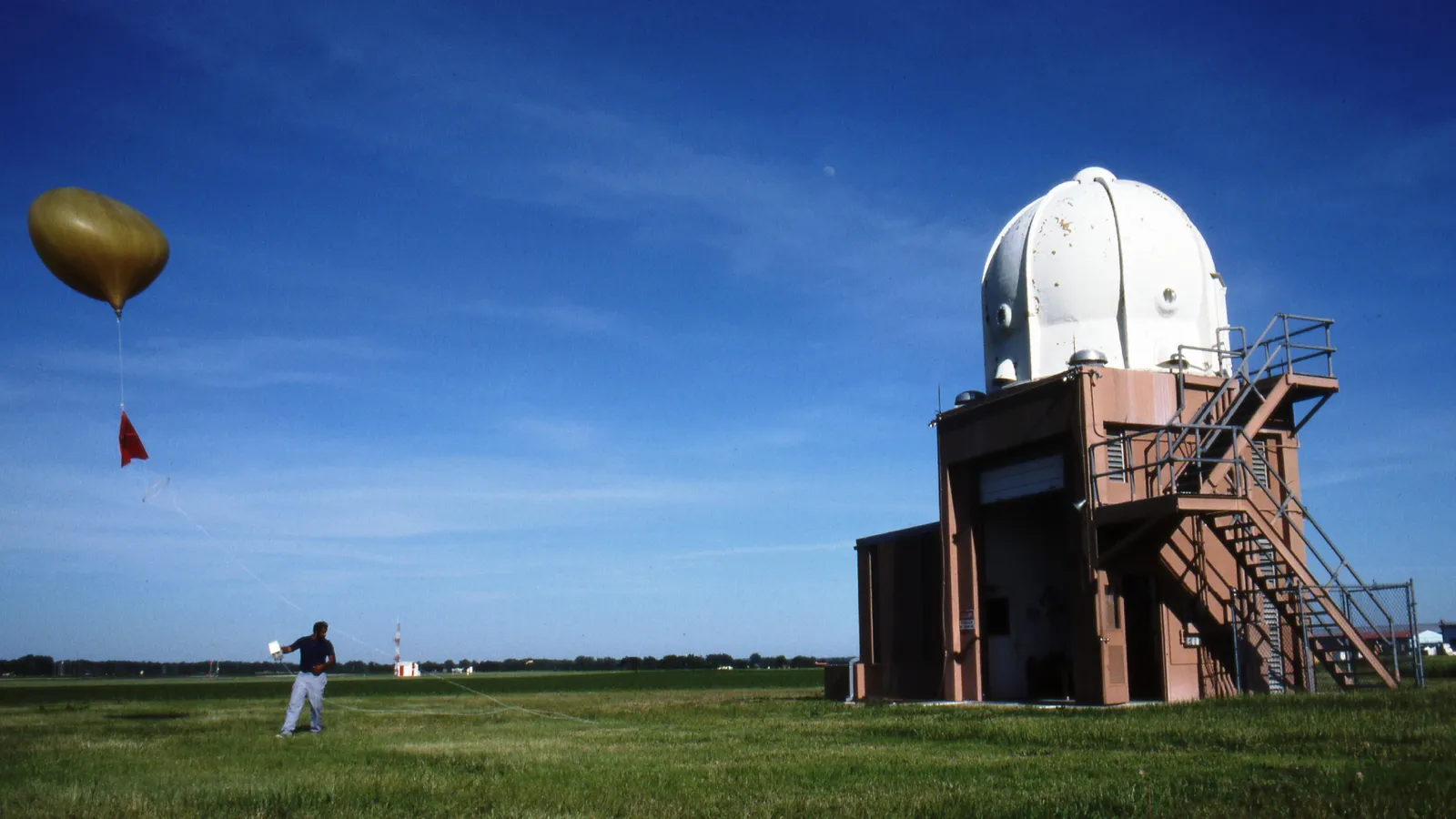
In meteorology a sounding is, in the American Meteorological Society's definition, the same as an upper-air observation, with the common connotation of "a single complete set of radiosonde observations."[2] The radiosonde is a small instrument package hung below a balloon filled with hydrogen or helium. As it rises at about 300 meters a minute (1,000 feet a minute), its sensors transmit pressure, temperature, relative humidity and GPS position every second. The wind is not measured directly; it is computed from how the radiosonde drifts, tracked by GPS.[1]
A flight lasts more than two hours, reaches more than 35 km (about 115,000 feet) and can drift more than 300 km from the launch site. The balloon leaves the ground about 1.5 m (5 feet) across and bursts at 6 to 8 m (20 to 25 feet), after which a small parachute brings the instrument down. No data are collected on the way down.[1]
| The US network | Figure |
|---|---|
| Stations | 92 |
| In the lower 48 states | 69 |
| Alaska / Pacific / Puerto Rico | 13 / 9 / 1 |
| Routine launch times | up to 1 hour before 00 and 12 UTC |
| In Central Daylight Time | about 6 am and 6 pm |
Launches happen at the same times every day of the year, up to an hour before 00 and 12 UTC, so the soundings from every station describe the same moment.[1] The times are named for the hour, in UTC: the "12Z sounding" is the morning one in the United States, the "00Z sounding" the evening one. On severe weather days offices launch extra balloons, usually at 18Z; two of the soundings in this lesson are 18Z specials.
Two consequences follow. A sounding is a snapshot of one column at one time, and a storm forming six hours later and 150 km away may sit in quite different air. And the balloon drifts downwind as it rises, so the upper part of the profile is measured tens of kilometers from the launch site. Forecasters fill the gaps with model soundings, which give the same profile for any place and hour, and which are the subject of a later lesson.
Why the chart is skewed
A skew-T log-P diagram is one of several thermodynamic diagrams, charts on which the gas laws and the first law of thermodynamics are built into the grid, so that the path of a rising or sinking parcel of air can be traced with a finger. The emagram, the tephigram and the Stüve diagram all "express the same physical relationships," in the words of the US Air Force manual on the skew-T, and all carry the same five families of lines.[3] The skew-T is, per the AMS, "an emagram (temperature and logarithm of pressure as coordinates) with the isotherms rotated 45° clockwise to produce greater separation of isotherms and dry adiabats."[2] Its coordinate system was first suggested by the Norwegian meteorologist N. Herlofson in 1947.[3]
The manual lists what a working diagram should do: keep the important lines straight, make the angle between the isotherms and the adiabats large enough to judge stability by eye, keep area proportional to energy everywhere on the chart, show a whole sounding into the stratosphere, and make height on the chart approximate height in the atmosphere. The skew-T is preferred over its close rivals "because its isobars are straight, which makes it easier to estimate pressure altitudes."[3]
The logarithmic pressure axis has two effects. Pressure falls roughly exponentially with height, so equal distances on a log scale are roughly equal distances in the atmosphere: the chart is close to a height chart, squeezed slightly at the top. And with both axes chosen this way, "a given area can be considered proportional to a certain amount of kinetic energy of a vertically and adiabatically moving air parcel."[3] That property is why CAPE and CIN, the energy available to a storm and the energy holding it back, are drawn and read as areas.
The five families of lines
Every skew-T carries the same background, whatever the colors. Each family answers one question about air that moves up or down.
- Isobars
- Horizontal lines of constant pressure, spaced logarithmically. They are the vertical axis: 1000 hPa is near sea level, 850 hPa about 1.5 km up, 500 hPa about 5.5 km, 250 hPa near the jet stream.[3]
- Isotherms
- Straight lines of constant temperature, sloping up to the right at 45 degrees and evenly spaced. A temperature is read along its isotherm, never straight down to the bottom axis.[3]
- Dry adiabats
- Gently curved lines sloping up to the left: the temperature of unsaturated air lifted or lowered with no heat added or removed. Air on them cools about 9.8 °C per kilometer as it rises. Each is also a line of constant potential temperature, labeled with its temperature at 1000 hPa.[2][3]
- Saturated adiabats
- Curved lines, dashed here, for saturated rising air. Condensation releases heat, so they cool more slowly than the dry adiabats near the ground, around 5 °C per kilometer in warm air, and become nearly parallel to them in the cold upper troposphere.[3][8] They assume the condensed water falls out at once, which is why they are also called pseudoadiabats.
- Mixing ratio lines
- Dotted lines of constant saturation mixing ratio, in grams of water vapor per kilogram of dry air, sloping up to the right more steeply than the isotherms. Read through the dew point, they give how much water vapor the air holds; read through the temperature, how much it could hold.[3]
Two of these families describe the atmosphere as it is (isobars and isotherms, the frame the measurements are plotted in). The other three describe what would happen to air if it moved: the dry adiabats, the saturated adiabats and the mixing ratio lines are paths, and reading a sounding mostly means comparing the measured profile with those paths.
Reading the traces
A plotted sounding adds two lines and a column of wind barbs. The temperature is always the right-hand trace. The dew point, the temperature at which the air would become saturated, is the left-hand one, and it can never lie to the right of the temperature. The horizontal gap between them, read along the isotherms, is the dew point depression: where the traces touch, the air is saturated, which usually means cloud; where they are far apart, the air is dry.
Table: the Norman sounding, 18 UTC May 20, 2013, at the surface and mandatory levels
| Pressure, hPa | Height above ground, m | Temperature, °C | Dew point, °C | Wind from, ° | Speed, kt |
|---|---|---|---|---|---|
| 966 | 0 | 27.4 | 22.4 | 185 | 10 |
| 925 | 385 | 22.8 | 18.6 | 185 | 16 |
| 850 | 1,116 | 16.6 | 14.6 | 215 | 29 |
| 700 | 2,758 | 9.6 | -6.4 | 225 | 42 |
| 500 | 5,425 | -11.7 | -27.7 | 240 | 54 |
| 400 | 7,105 | -23.5 | -39.5 | 245 | 55 |
| 300 | 9,135 | -39.9 | -58.9 | 250 | 62 |
| 250 | 10,355 | -49.3 | -70.3 | 250 | 67 |
| 200 | 11,795 | -54.7 | -71.7 | 255 | 71 |
| 150 | 13,645 | -54.7 | -72.7 | 245 | 30 |
| 100 | 16,165 | -64.7 | -78.7 | 195 | 21 |
Three reading habits prevent most mistakes. Read temperature along the tilted isotherm through the point, not straight down: the orange trace at 500 hPa sits above about 14 on the bottom axis, but its temperature is −11.7 °C. Judge moisture by the gap between the traces, not by the dew point alone: −6.4 °C at 700 hPa is dry air even though the number looks mild. And read slopes against the background lines, not against the page: a trace that looks vertical on a skew-T is cooling with height at roughly the moist adiabatic rate.
Wind barbs
The barbs down the right edge give the wind at each level. The staff points toward the direction the wind is blowing from. A half barb is 5 knots, a full barb 10, a triangular flag 50; they add up. A wind that strengthens and turns clockwise with height, as it does on the Norman sounding, is the signature of the vertical wind shear that organizes supercells. The hodograph, the subject of the next lesson in the unit, draws the same winds as a single curve.
Lapse rates and stability
The lapse rate is the rate at which temperature falls with height. Stability is decided by comparing the measured lapse rate with the rate a displaced parcel would follow. Unsaturated air cools at the dry adiabatic rate, "approximately 9.8°C km⁻¹."[2] Saturated air cools more slowly, at a rate that depends on temperature; a typical value is around 5 °C per kilometer.[8]
- Temperature profile
- Dry adiabat through the start
- Saturated adiabat through the start
- Absolutely unstable
- The lapse rate exceeds the dry adiabatic rate. Air displaced up or down "would be accelerated in the direction of the displacement." It occurs in a thin layer over hot ground on sunny afternoons and does not last, because the air overturns.[2]
- Conditionally unstable
- The lapse rate lies between the moist and dry rates. The layer is stable for unsaturated air and unstable for saturated air: air that is lifted until it condenses can then rise on its own.[2] This is the normal state of the atmosphere on a thunderstorm day.
- Absolutely stable
- The lapse rate is less than the moist rate. Lifted air, saturated or not, is denser than its surroundings "and would tend to sink back to its level of origin."[2]
Forecasters summarize the middle troposphere with the 700 to 500 hPa lapse rate. NWS Houston/Galveston's training page gives a rule of thumb: under 5.5 °C per kilometer is stable and 5.5 to 9 conditionally unstable.[6] Values near 8 or more are steep and usually mean a plume of air that was heated over higher ground to the west. On the Norman sounding the layer measured 8.5 °C per kilometer at 7 am.
Inversions and the cap
An inversion is a layer in which temperature rises with height, and on a skew-T the temperature trace bends to the right through it. The Air Force manual describes three common kinds, each with its own signature in the dew point.[3]
- Radiation inversions form on clear, calm nights as the ground cools the air in contact with it; their depth depends on wind, cloud and the length of the night. They sit at the ground and are where fog forms.
- Subsidence inversions form where a deep layer of air has sunk and warmed by compression. Their mark is "a strong upward decrease of moisture through the inversion," and the manual names the California coastal inversion as an example that "persists for long periods in the summer."
- Frontal inversions mark the boundary between a cold air mass below and a warmer one above; more often they appear as a shallow isothermal or very stable layer, with the dew point rising through it.
The inversion that matters most on a severe weather day is the cap: a stable layer above the moist air near the ground that traps heat and moisture beneath it. In the southern Plains it is usually the base of a layer of hot, dry air that was heated over higher terrain to the west and southwest and has flowed east over the moist Gulf air. NWS Houston/Galveston's training material: "This hot dry air originates at higher elevations it will stay around that higher elevation as it moves east," and "the hot and dry air creates a cap." A cap that is too strong produces a bust, a day with every ingredient and no storms; one that is too weak lets storms form early and compete with each other. "Once the CAP is broken, explosive development of thunderstorms can occur."[7]
Lifting a parcel: the cloud base
Everything that follows comes from one procedure: take a sample of air, an air parcel, lift it on the chart, and compare its temperature with the air around it at every level. Two things stay constant as unsaturated air rises: its potential temperature, so it follows a dry adiabat, and its moisture content, so its dew point follows a mixing ratio line.
The meeting point is the lifted condensation level, the LCL: in the AMS definition, the level at which moist air lifted dry-adiabatically "would become saturated," located "at the point of intersection of the dry adiabat through the point representing the parcel's original pressure and temperature with the saturation mixing ratio line having the same value of the mixing ratio as the parcel."[2] It is the base of the clouds that lifted air produces. The drier the air, the further apart the traces start and the higher the base: at Denver on the afternoon of the microburst described below, the LCL was 4,400 m above the ground.
A related level asks how warm the ground has to get before heating alone makes clouds. Follow the mixing ratio line up from the surface dew point until it meets the temperature trace: that is the convective condensation level. The dry adiabat through it, followed back down to the ground, gives the convective temperature: "the surface temperature that must be reached to start the formation of convection clouds by solar heating."[3] The University of Wyoming's analysis of the 7 am Norman sounding puts it at 35.8 °C (96 °F).[4]
LFC, EL, CAPE and CIN
Above the LCL the parcel follows the saturated adiabat, and the question becomes whether it is warmer than the surrounding air. Warmer air is less dense and accelerates upward; cooler air is denser and has to be pushed.
- Temperature
- Dew point
- Lifted parcel
- CIN
- CAPE
Table: the Norman sounding, 12 UTC May 20, 2013, at the surface and mandatory levels
| Pressure, hPa | Height above ground, m | Temperature, °C | Dew point, °C | Wind from, ° | Speed, kt |
|---|---|---|---|---|---|
| 966 | 0 | 21.6 | 19.7 | 160 | 7 |
| 925 | 372 | 20 | 19 | 195 | 34 |
| 850 | 1,108 | 22.6 | 4.6 | 220 | 24 |
| 700 | 2,755 | 8.6 | -8.4 | 220 | 25 |
| 500 | 5,415 | -14.1 | -24.1 | 250 | 45 |
| 400 | 7,095 | -22.7 | -51.7 | 245 | 53 |
| 300 | 9,135 | -37.9 | -58.9 | 250 | 56 |
| 250 | 10,365 | -48.7 | -63.7 | 240 | 52 |
| 200 | 11,795 | -54.7 | -67.7 | 250 | 69 |
| 150 | 13,645 | -55.5 | -68.5 | 265 | 41 |
| 100 | 16,165 | -63.5 | -74.5 | 310 | 21 |
| Surface parcel CAPE, J/kg | 1,829 | ||||
| Surface parcel CIN, J/kg | -271 | ||||
| LCL / LFC / EL, hPa | 939 / 713 / 206 | ||||
- LFC
- The level of free convection: where the lifted parcel "would first become warmer than its surroundings in a conditionally unstable atmosphere." Above it, the parcel rises on its own.[2]
- EL
- The equilibrium level: where the rising parcel "attains the same density as its environment." Updrafts decelerate above it; the anvil spreads out near it, and an overshooting top marks an updraft carried past it.[2]
- CAPE
- Convective available potential energy: the area between the parcel and the temperature trace from the LFC to the EL, where the parcel is warmer. It "can be viewed as the maximum kinetic energy that could be gained by a rising air parcel due to work done by buoyancy," and is the standard measure of how strong updrafts can become.[2]
- CIN
- Convective inhibition: the area where the parcel is cooler than its surroundings below the LFC, the energy "needed to lift an air parcel" to its LFC. "If convective inhibition is sufficiently large, deep convection will not form."[2]
Both are given in joules per kilogram. NWS Houston/Galveston's training page grades CAPE as positive up to 1,500 J/kg, large from 1,500 to 2,500 and extreme above 2,500.[6] CIN has no such scale; what matters is whether heating, moisture or a front, dryline or outflow boundary can supply the energy to overcome it. Neither number means much without the other. A 7 am sounding with 1,829 J/kg of CAPE and −271 J/kg of CIN, like this one, says that a great deal of energy is available and that nothing will use it yet.
How the cap breaks
Six hours later the same station launched again. The difference between the two soundings is the most important thing a forecaster watches on a capped day.
Three things erode a cap, and a sounding shows each. Heating at the ground moves the start of the parcel's path to the right, onto a warmer dry adiabat that clears the inversion. Added moisture at the ground lowers the LCL and puts the parcel on a warmer saturated adiabat. And rising air on a large scale, ahead of an upper-level trough, cools the layer aloft and weakens the inversion itself. On May 20 the first two are plain in the two soundings. The Moore tornado touched down at 2:56 pm CDT, about two hours after the second launch.[15]
Which parcel to lift
CAPE and CIN depend on which air is lifted, and the Air Force manual says so directly: the areas "are not uniquely defined on any given sounding. They depend on the parcel chosen."[3] The Storm Prediction Center reports three, each with the virtual temperature correction for the lower density of moist air.[5]
| Parcel | Starting air | Norman, 1 pm, CAPE J/kg | CIN J/kg |
|---|---|---|---|
| Surface-based | The air at the ground | 4,892 | 0 |
| Mixed-layer | The average of the lowest 100 hPa | 2,920 | −5 |
| Most-unstable | The most buoyant air in the lowest 300 hPa | 4,892 | 0 |
The surface parcel is the warmest and moistest air of the afternoon, but a real updraft draws on a deeper layer, and the mixed-layer parcel represents that better; it is the one the Storm Prediction Center's tornado parameters use. The spread between the two is itself information: here the surface air is much more buoyant than the layer above it, which is typical of a hot afternoon. Small choices in the averaging matter too. The tornado lesson gives this sounding 3,117 J/kg of mixed-layer CAPE, from an average of the reported levels; weighting the layer by pressure, as here, gives 2,920.[16] Treat CAPE values as good to a few hundred joules per kilogram, and compare numbers only when they were computed the same way.
The most-unstable parcel matters when the best air is not at the ground. Storms that form above a layer of cold air, north of a warm front or in winter, are called elevated: they draw their air from above the inversion and cannot use the stable air beneath. Colman (1990), as summarized by Bradford Grant, found that "nearly all cool season (Nov-Feb) thunderstorms east of the Rockies, with the exception of those over Florida, were of the elevated type."[10]
Table: the Topeka sounding, 12 UTC April 9, 1992, at the surface and mandatory levels
| Pressure, hPa | Height above ground, m | Temperature, °C | Dew point, °C | Wind from, ° | Speed, kt |
|---|---|---|---|---|---|
| 982 | 0 | 8.2 | 6.3 | 40 | 15 |
| 925 | 500 | 11.4 | 9.9 | 55 | 21 |
| 850 | 1,212 | 11.2 | 10.2 | 295 | 5 |
| 700 | 2,802 | 0.8 | -11.2 | 230 | 19 |
| 500 | 5,412 | -17.3 | -30.3 | 270 | 35 |
| 400 | 7,042 | -30.5 | -43.5 | 280 | 38 |
| 300 | 9,022 | -47.1 | 275 | 45 | |
| 250 | 10,202 | -56.1 | 275 | 50 | |
| 200 | 11,592 | -66.3 | 265 | 58 | |
| 150 | 13,322 | -64.3 | 280 | 64 | |
| 100 | 15,842 | -60.5 | 270 | 64 |
Six sounding shapes
With practice a sounding's shape says what kind of day it is before any number is computed. The six below are real soundings, each launched near a documented event.
- Temperature
- Dew point
- 0 °C isotherm
Loaded gun
A moist layer at the ground, a sharp cap above it, and above the cap a deep, dry layer with a steep lapse rate: the classic severe weather sounding, listed on NWS Houston/Galveston's training page as "Severe weather sounding (large CAPE, very unstable LI)."[6] The cap stores the energy and the steep layer above it makes the energy large; when the cap breaks, the release is sudden. The Norman sounding of May 20, 2013 is the example.
Inverted V
The temperature and dew point spread apart toward the ground, forming an upside-down V: a deep, dry, well-mixed layer under a moist layer aloft. The Houston/Galveston page describes it as "dry air (low RH) in lower troposphere with nearly saturated air (high RH) in middle troposphere."[6] Rain falling from high-based storms evaporates in the dry layer, cools the air and drives it down hard: the setup for dry microbursts, often with little rain at the ground and virga overhead. On June 10, 2013, storms moved off the Front Range "into a region with a deep, unstable mixed layer below the 500-mb level," and at 2120 UTC a microburst produced an 80 mph gust 10 miles east of Parker, Colorado.[11] The Denver sounding launched about two hours later has a surface temperature of 34.6 °C, a dew point of −1.4 °C, and a cloud base 4,400 m above the ground.
Saturated tropical column
The two traces lie on top of each other from the ground to the upper troposphere: moist through its whole depth, with a lapse rate close to the saturated adiabat and little CAPE. Such soundings produce extreme rainfall rates rather than severe storms. The Corpus Christi sounding launched as Hurricane Harvey approached, at 00 UTC August 26, 2017, measured 2.78 inches of precipitable water, the highest on record for August at the station, according to Weather Underground's account of the storm.[12] Integrated here to 300 hPa, the same sounding gives 2.74 inches.
Warm nose
In winter the question is what falls, and it is answered by where the temperature trace crosses 0 °C. A layer above freezing aloft, the warm nose, melts snow falling through it; what happens next depends on the cold layer beneath. A shallow cold layer lets the drops reach the ground as liquid and freeze on contact: freezing rain. A deep one refreezes them into ice pellets: sleet.[8] The Fort Worth sounding at 6 pm CST December 5, 2013 has a warm layer peaking at 7.8 °C near 2 km over a subfreezing layer about 800 m deep, as cold as −6.5 °C. Freezing rain, sleet and a little snow fell through the next morning, and "sleet and ice measured as deep as 5" in some areas."[13]
Snow
When the whole profile stays below 0 °C, snow reaches the ground as snow. The saturated layer's temperature then decides the kind of crystal. Forecasters look for saturated air in the "dendritic layer" from −12 to −18 °C, "centered around −15C," where snow production is most efficient.[8] The Great Falls, Montana sounding during the storm of November 8 to 10, 2012 is saturated and below freezing from the ground up; the National Weather Service's study of the storm tracked how the depth of that growth zone changed through the event and with it the snow-to-liquid ratio, which averaged 14 to 1.[14]
Marine layer
A cool, moist layer at the ground, capped by an abrupt, strong inversion with very dry air above it: the subsidence inversion of the California coast. At Oakland on the morning of July 15, 2024 the marine layer was about 550 m deep, and through the next 170 m the temperature rose 12.6 °C while the dew point fell from 10.4 to −11 °C. Stratus and fog form in the moist layer, and the inversion keeps them there until the sun or the wind mixes them out.[3][4]
Stability indices
Sounding pages list single-number indices computed from a few levels. They predate the computers that now lift parcels through the whole profile, and they are useful as a quick read and misleading as a verdict. Their thresholds come from different places and disagree, so both common versions are given here.
| Index | What it is | Air Force manual / AMS | NWS Houston/Galveston | Norman, 7 am |
|---|---|---|---|---|
| Lifted index | 500 hPa temperature minus a lifted parcel's there | 0 to −2 possible, needs a trigger; −3 to −5 probable; below −5 very unstable | −1 to −4 marginal; −5 to −7 large; −8 to −10 extreme | −9.2 |
| K index | 850−500 hPa temperature difference plus moisture at 850 and 700 hPa | Thunderstorm likelihood rises from about 20 | 15 to 25 small; 26 to 39 moderate; 40 or more high potential | 24.3 |
| Total totals | 850 hPa temperature plus dew point, minus twice the 500 hPa temperature | Convection threshold 44; over 55 strong thunderstorm potential | 44 to 50 convection likely; over 56 scattered severe | 55.4 |
| Precipitable water | All the water vapor in the column, as a depth of liquid | No threshold given | Over 1.75 in water-loaded; under 0.75 in fairly dry | 1.02 in |
Sources: the Air Force manual for the lifted index and total totals, the AMS glossary for the K index, and the Houston/Galveston training page. The Norman column is computed here from the 12 UTC sounding, with the lifted index taken from the mixed-layer parcel.[2][3][6] The manual's own caution applies to all of them: "these values will vary with seasons, locations, and synoptic settings," and the K index in particular is biased toward ordinary summer storms because it rewards moisture at 700 hPa.[3] The last column shows why. On the morning of the Moore tornado the K index read 24, "small potential" on the Houston scale, because the dry air at 700 hPa counts against it; that same dry layer above the cap was part of what made the day dangerous. None of these indices measures wind shear, which decides whether storms rotate.
Reading a sounding page
The Storm Prediction Center publishes every observed sounding in the country as a skew-T with a hodograph and a panel of computed parameters, with a seven-day archive, produced with its sounding analysis program.[9] The University of Wyoming keeps an archive of observed soundings going back decades, as tables, charts and indices.[4]

A reading order
With a sounding in front of you, this order covers what matters before any detail.
- Where and when. Station, date and time in UTC, and whether it is observed or from a model. Then ask how far it is, in time and distance, from the weather you care about.
- Moisture. Surface dew point, and the depth of the moist layer: how far up the traces stay close together. Note dry layers aloft.
- Temperature structure. Inversions and where they are, the 700 to 500 hPa lapse rate, and the 0 °C level.
- The parcel. Lift it, with mixed-layer as the default, and read the LCL, LFC, EL, CAPE and CIN. Compare with the surface and most-unstable parcels.
- What changes it. How much heating or moisture would remove the CIN; whether the layers above are forecast to cool or warm.
- Wind. Speed and direction with height, and whether they strengthen and turn. Then open the hodograph.
Check yourself
-
On a skew-T, the temperature trace at 500 hPa sits directly above the 14 on the bottom axis. Is the temperature 14 °C?
Answer
No. Temperature is read along the isotherm through the point, which slopes up to the right at 45 degrees. On the Norman sounding chart above, that point is −11.7 °C.
-
The temperature and dew point traces touch from 850 to 700 hPa and are 20 °C apart above. What is most likely at 850 to 700 hPa?
Answer
A saturated layer: cloud. Above it the air is dry.
-
How do you find the lifted condensation level?
Answer
Follow the dry adiabat up from the surface temperature and the mixing ratio line up from the surface dew point. The LCL is where they meet.
-
A morning sounding shows 2,000 J/kg of CAPE and −300 J/kg of CIN. Will storms form?
Answer
Not as it stands. The energy is there but the cap is strong. Storms need heating, added moisture, cooling aloft or a boundary to lift the air; the afternoon sounding or a model forecast is needed to judge whether the CIN will be removed.
-
Surface-based CAPE is zero but most-unstable CAPE is 1,000 J/kg. What does that mean?
Answer
The unstable air is above a stable layer at the ground, typically north of a front. Storms that form will be elevated, drawing their air from above the inversion; their main hazard is usually hail.
-
The temperature rises above 0 °C between 900 and 750 hPa and is −5 °C at the ground. What falls?
Answer
Snow melts in the warm layer. If the cold layer below is shallow, freezing rain; if it is deep, sleet. Here the cold layer is roughly the lowest 1 km, so sleet or a mix is likely.
Video


Methods
Every sounding here is the observed radiosonde record from the University of Wyoming's
archive, plotted and analyzed by WeatherOverTime's own code. Saturation vapor pressure is
from Bolton (1980); parcels are lifted dry-adiabatically to saturation and then along a
pseudoadiabat integrated in 1 hPa steps, without ice or water loading; CAPE and CIN use
virtual temperature for both the parcel and the environment. The LFC is the first level
above the LCL at which the parcel is warmer than its surroundings, the EL the top of the
highest positive layer, CAPE every positive area between them and CIN every negative area
below the LFC. The mixed-layer parcel averages potential temperature and mixing ratio over
the lowest 100 hPa, weighted by pressure; the most-unstable parcel is the level of highest
equivalent potential temperature in the lowest 300 hPa. For the 7 am Norman sounding this
gives a most-unstable CAPE of 4,458 J/kg against the University of Wyoming's 4,435.
Precipitable water is integrated from the surface to 300 hPa. The lapse rate panels are
idealized. The code and the soundings are in the site's repository, under
scripts/learn/.
Related
The ingredients read here are put to work in How tornadoes form, which walks through the soundings before nine tornadoes. The Moore tornado of the Norman soundings has its own profile, with the radar replayable scan by scan. In Storm Lab, a storm can be grown from an observed sounding. Unfamiliar terms are in the glossary.
Sources
Quotations are verbatim from the source named. The Air Force manual was read from an optical character recognition copy; quotations from it were checked against the column order of the page. Figures marked "computed here" are described under Methods.
- National Weather Service, Radiosonde Observation, upper-air fact sheet.
- American Meteorological Society, Glossary of Meteorology, entries sounding, skew T–log p diagram, dry-adiabatic lapse rate, absolute instability, conditional instability, absolute stability, lifting condensation level, level of free convection, level of neutral buoyancy, convective available potential energy, convective inhibition and stability index.
- Air Weather Service, The Use of the Skew T, Log P Diagram in Analysis and Forecasting, AWS/TR-79/006, revised 1990: chapters 1 and 2 (the diagram and its lines), paragraphs 4.18 to 4.24 (CCL, convective temperature, LCL, LFC, EL, energy areas), 5.24 (indices) and chapter 6 (inversions). Copy hosted by the University of Arizona. It cites N. Herlofson, "The T, log p-Diagram with Skew Coordinate Axes," Meteorologisk Annaler 2 (10), 1947.
- University of Wyoming, Department of Atmospheric Science, upper-air soundings: Norman, OK (72357) 12 and 18 UTC May 20, 2013; Denver, CO (72469) 00 UTC June 11, 2013; Corpus Christi, TX (72251) 00 UTC August 26, 2017; Fort Worth, TX (72249) 00 UTC December 6, 2013; Great Falls, MT (72776) 00 UTC November 9, 2012; Oakland, CA (72493) 12 UTC July 15, 2024; Topeka, KS (72456) 12 UTC April 9, 1992. Indices as published with the Norman 12 UTC sounding.
- Storm Prediction Center, mesoanalysis help: surface-based CAPE, mixed-layer CAPE, most-unstable CAPE.
- National Weather Service Houston/Galveston, Skew-T parameters and indices, training page.
- National Weather Service Houston/Galveston, Temperatures: The Inversion, training page.
- Mark A. Rose, National Weather Service Nashville, The Skew-T Log P Diagram, training slides: lapse rates (slide 4), the dendritic growth layer (slide 21) and winter precipitation types (slides 25 to 29).
- Storm Prediction Center, Observed Soundings.
- Bradford N. Grant, Elevated Cold-Sector Severe Thunderstorms: A Preliminary Study, National Weather Digest 19 (4), 1995, including its summary of Colman (1990).
- Ken Pryor, Dan Bikos and Scott Lindstrom, VISIT Meteorological Interpretation Blog, 10 June 2013 Colorado dry microburst, CIRA, Colorado State University.
- Jeff Masters and Bob Henson, Weather Underground Category 6, Heavy damage in Texas; Harvey now a tropical storm, August 26, 2017.
- National Weather Service Fort Worth, December 5 to 10, 2013 winter storm.
- National Weather Service Western Region, Snow-to-Liquid Ratios Associated with a Strong November Snowstorm, Technical Attachment 16-04.
- WeatherOverTime, Moore, Oklahoma tornado, May 20, 2013, and its sources.
- WeatherOverTime, How tornadoes form, methods.
- Stephen Corfidi, NOAA/NWS/SPC, NOAA Photo Library image wea01144, Launching a weather balloon radiosonde, Topeka, Kansas, May 26, 1988, public domain.
- Storm Prediction Center, Lake Charles sounding, 18 UTC December 16, 2019, via Wikimedia Commons, public domain.
- NWS Billings, Introduction to the Skew-T Log P Diagram, YouTube.
- Storm Chaser Gabe Garfield, How to Read Skew-T Log-p Charts, For Beginners, YouTube.
- Alex Schoel WX, Understanding Weather Soundings: How to Read a Skew-t chart, YouTube.
- Matthew Dehr, Basic Instructions for Interpreting a Skew-T Chart for Severe Weather Days, YouTube.


Corrections: contact@weatherovertime.com.
Unit 5: Soundings
- How to read a skew-T diagram
Every line on the chart, how to lift a parcel, CAPE and CIN, and the sounding shapes behind storms, snow, ice and fog.
- How to read a hodograph
The wind profile as one curve: shear, turning, storm motion and helicity.
- Severe weather parameters
What STP, SCP, SRH and effective shear measure, and what their thresholds mean.
- Forecast soundings from models
Reading model soundings, and where they are most often wrong.