Vorticity
- Read first
- Air pressure
- Key terms
- Vorticity, Relative vorticity, Absolute vorticity, Coriolis parameter, Circulation, Vorticity advection, Level of nondivergence, Shortwave trough, Vortex stretching, Potential vorticity, Lee trough, Lee cyclogenesis, Colorado low, Tilting term, Streamwise vorticity, Helicity, Storm-relative helicity, Mesocyclone, Dynamic tropopause, Tropopause fold
Every low-pressure system, every trough on the 500 hPa chart and every rotating thunderstorm spins, and meteorologists measure that spin with one quantity: vorticity. This lesson explains what it is, where it comes from, how it is computed from real winds and why the places where it is largest, and where the wind carries it, are where weather happens. The example running through it is the storm of March 13, 2019, which formed in the lee of the Rocky Mountains and set Colorado's record for low pressure. The lesson then follows the spin down in scale, to the horizontal vorticity in the winds of a tornado day in Oklahoma, the mesocyclone and the tornado itself.
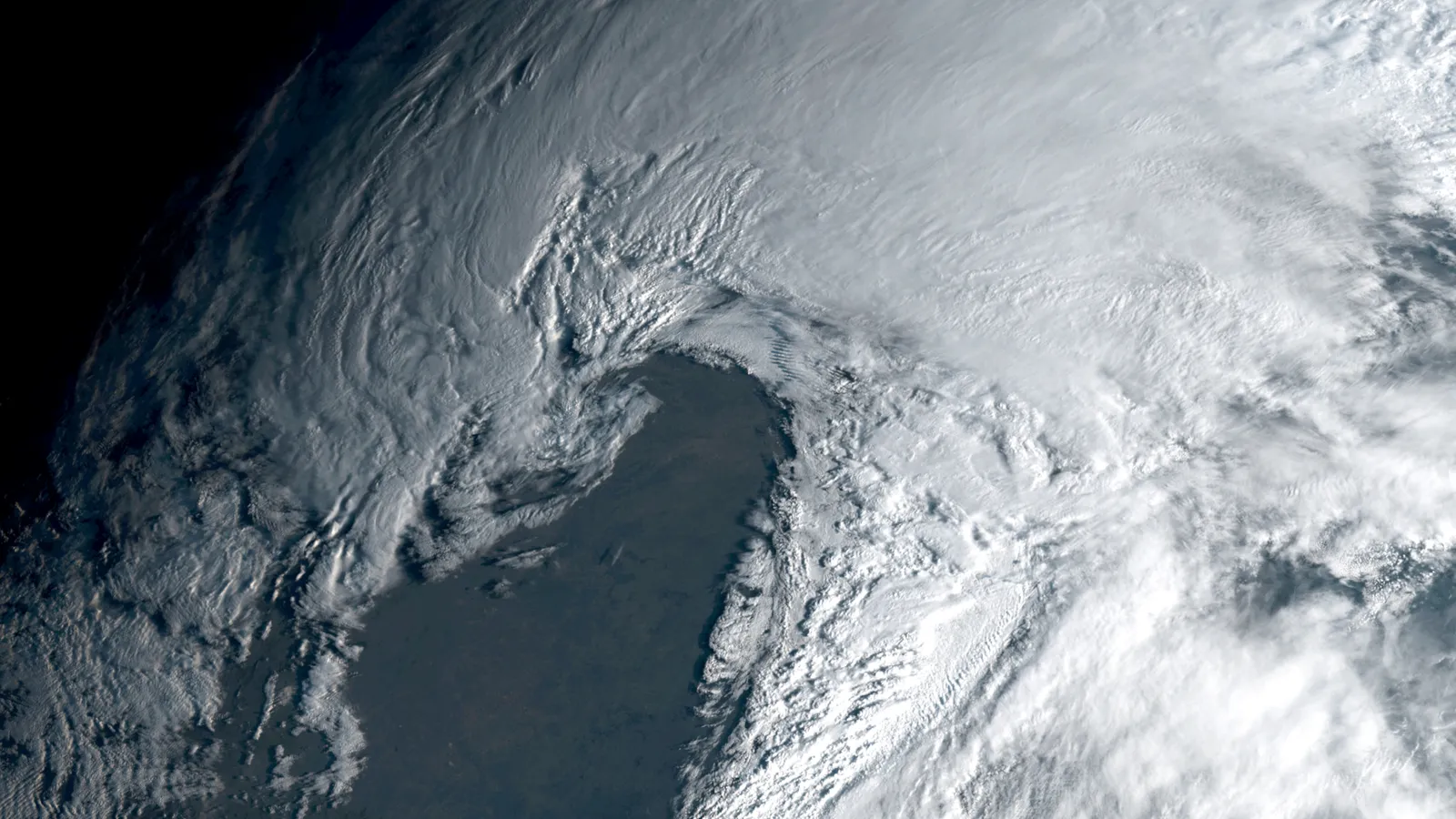
- What vorticity is: the curl of the wind, its sign, and its two sources, shear and curvature.
- The Earth's own spin, the Coriolis parameter f, and absolute vorticity.
- Computing it from real winds: a grid of analyzed winds, and six balloon soundings around a storm.
- The 500 hPa vorticity map, vorticity maxima as the mark of shortwaves, and vorticity advection.
- Conservation: why stretching spins air up, why a trough forms east of the Rockies, and the Colorado low of March 2019.
- From the environment to the storm: horizontal vorticity, tilting, the mesocyclone and the tornado, and potential vorticity at the tropopause.
What vorticity is
The American Meteorological Society defines vorticity as "a vector measure of local rotation in a fluid flow, defined mathematically as the curl of the velocity vector." In meteorology, "'the vorticity' usually refers to the vertical component of the vorticity," the spin about an axis pointing straight up.[1] The curl is a way of asking, at every point, whether the air around that point is turning. Picture a small paddle wheel with a vertical axle, carried along by the wind. If the wind pushes harder on one side of it than the other, it spins; vorticity is how fast.
On a map, with x pointing east, y north, and the wind's eastward and northward components u and v, the vertical component is
ζ = ∂v/∂x − ∂u/∂y
In words: the northward wind increasing toward the east turns a paddle wheel counterclockwise, and so does an eastward wind that weakens toward the north. The two terms are the two ways air can turn a wheel, and they add. Carl-Gustaf Rossby wrote exactly this in 1939, with his convention: "Vorticity is counted positive for cyclonic rotation, negative for anticyclonic rotation."[5]
Relative vorticity, written ζ (zeta), is "the vorticity as measured in a system of coordinates fixed on the earth's surface." Cyclonic means "having a sense of rotation about the local vertical the same as that of the earth's rotation": counterclockwise seen from above in the Northern Hemisphere, clockwise in the Southern.[1] In the Northern Hemisphere, then, lows and troughs have positive vorticity and highs and ridges negative. Southern Hemisphere cyclones turn clockwise and have negative relative vorticity; the sign follows the direction of the Earth's own turn, and flips across the equator.
Two more statements in the AMS definition help. "The vorticity of a solid rotation is twice the angular velocity": a turntable spinning at one radian per second has a vorticity of 2 per second. And the vorticity across a small area "is the limit of the circulation per unit area," the total flow around the edge of the area divided by the area itself.[1] That second form is how vorticity is measured from scattered observations later in this lesson. Its unit is per second, s⁻¹. Weather maps print it in units of 10⁻⁵ s⁻¹, so a "12" on a 500 hPa chart means 12 × 10⁻⁵ s⁻¹.[3]
Shear and curvature
Air picks up relative vorticity in two ways. NOAA's JetStream course describes both with a stick floating in a river.[2]
- Shear vorticity
- "The rate at which the water flows down the center of the river is faster than near the shore," so the end of the stick nearer the middle moves faster and the stick turns. "Looking downstream, if the stick is to the left of centerline, then the rotation will be counter clockwise." In the atmosphere, "a parcel located on the north side of the jet stream will experience increased counter clockwise flow," and one south of it clockwise flow.[2]
- Curvature vorticity
- Where the river bends, a stick lying across it turns to keep its orientation to the bank. "For the Northern Hemisphere atmosphere, parcels of air will have cyclonic (counter clockwise) spin in troughs and anti-cyclonic (clockwise) spin in ridges."[2]
Roland Stull's Practical Meteorology writes the same split for air turning around a center: with a tangential wind M at a distance R from the center, ζ = ΔM/ΔR + M/R, the first term the shear and the second the curvature. For a solid rotation the two are equal and ζ = 2M/R, which is the AMS's "twice the angular velocity" again.[4][1] The two parts can also cancel. Air curving cyclonically around the south side of a trough while the wind weakens toward the trough's center can have almost no net vorticity, and a jet stream running straight across a map has strong vorticity on both flanks with no curvature at all. The map shows the sum; the words "shear" and "curvature" are a way of reading where it came from.
The Earth's spin and absolute vorticity
Air at rest on the ground is not at rest in space: it turns with the Earth. The part of that turning about the local vertical is the Coriolis parameter, f, "twice the component of the earth's angular velocity about the local vertical, 2Ω sin φ," where Ω is the Earth's rate of rotation and φ the latitude. "Since the earth is in rigid rotation, the Coriolis parameter is equal to the component of the earth's vorticity about the local vertical."[1] JetStream calls it planetary vorticity: "At the poles, this vorticity is at its maximum, and it decreases as one moves toward the equator."[2]
| Latitude | f, 10⁻⁵ s⁻¹ | A disk at rest on the ground turns once in |
|---|---|---|
| 0° (equator) | 0 | never |
| 10° | 2.53 | 138 hours |
| 20° | 4.99 | 70 hours |
| 30° | 7.29 | 47.9 hours |
| 40° | 9.37 | 37.2 hours |
| 45° | 10.31 | 33.8 hours |
| 50° | 11.17 | 31.2 hours |
| 60° | 12.63 | 27.6 hours |
| 90° (pole) | 14.58 | 23.9 hours |
Computed here with Ω = 7.2921 × 10⁻⁵ s⁻¹. The last column turns the number into something physical: vorticity is twice the rate of turning, so the ground at latitude φ turns about the vertical at Ω sin φ, once every sidereal day (23.93 hours) divided by sin φ. At 40° N, where the storm in this lesson formed, a disk lying on the ground makes one full turn against the stars every 37 hours.
Adding the two gives absolute vorticity, "the vorticity of a fluid particle determined with respect to an absolute coordinate system," whose vertical component is the sum of the relative vorticity and the Earth's vorticity:[1]
η = ζ + f
In the Northern Hemisphere f is always positive, so absolute vorticity is usually positive too. It turns negative only where anticyclonic relative vorticity is larger than f, in small patches such as the strongest negative value on the map below. JetStream notes that the vorticity printed on 500 hPa charts is absolute vorticity, and "the largest vorticity values are found in troughs north of the jet stream, with the lowest values in ridges south of the jet stream."[2] Stull's worked example shows why the distinction matters: a west wind of 100 m/s at 50° N over one of 50 m/s at 46° N has a relative vorticity of −1.14 × 10⁻⁴ s⁻¹, almost exactly cancelling the Earth's 1.08 × 10⁻⁴ at 48° N, for an absolute vorticity near zero.[4]
Computing vorticity from real winds
The formula becomes a number once there are winds on a grid. The NCEP Global Forecast System's analysis for 12 UTC March 13, 2019, 6 am in Colorado, gives winds every half degree of latitude and longitude at 500 hPa.[7] At the grid point 37° N, 101.5° W, at the Oklahoma Panhandle's western edge, the four neighbors were:
| Neighbor | Distance from the point | Wind component |
|---|---|---|
| East, 101.0° W | 44.4 km | v = 46.1 m/s (from the south) |
| West, 102.0° W | 44.4 km | v = 23.2 m/s |
| North, 37.5° N | 55.6 km | u = −4.8 m/s (from the east) |
| South, 36.5° N | 55.6 km | u = 8.5 m/s (from the west) |
The south wind grew by 22.9 m/s across 88.8 km, so ∂v/∂x = 25.8 × 10⁻⁵ s⁻¹. The west wind fell from 8.5 m/s to −4.8 m/s going north across 111.2 km, so ∂u/∂y = −12.0 × 10⁻⁵ s⁻¹, and subtracting it adds another 12.0. A small term for the Earth's curvature adds 0.02. The total is 37.8 × 10⁻⁵ s⁻¹, four times the Earth's own vorticity there, 8.8 × 10⁻⁵. GFS's own analysis of the same point, computed inside the model, is 40.2. Computed here.
Both terms were cyclonic and the first was twice the second: air racing north on the east side of the point and turning back to the west on its north side, the wind of a closed low. Across the whole map the vorticity computed here this way differs from GFS's own by 2.5 × 10⁻⁵ s⁻¹ root mean square, most of it small-scale noise over the mountains.
The answer depends on the grid. The same calculation on the NCEP/NCAR Reanalysis, whose grid points are 2.5° apart, gives a largest value of only 13.1 × 10⁻⁵ s⁻¹ for the same storm at the same hour.[8] A difference taken across 280 km cannot see a gradient that is concentrated in 90. Vorticity maxima are compact, and a quoted value means little without the spacing it was measured over. Computed here.
The analysis is itself built from observations. Vorticity can be computed from the observations directly, through the second part of the AMS definition: the circulation around a closed curve, "a precise measure of the average flow of fluid along a given closed curve," equals "the total vorticity of the fluid enclosed by the curve."[1] Add up the wind along the edges of a loop, divide by the area inside, and the result is the average vorticity of the air within.
Table: the 500 hPa winds and the circulation, leg by leg, 12 UTC March 13, 2019
| Leg | Length, km | Mean wind along the leg, m/s | Contribution, 10⁶ m²/s |
|---|---|---|---|
| ABQ to AMA | 431 | 22.8 | 9.8 |
| AMA to DDC | 320 | 32.2 | 10.3 |
| DDC to LBF | 380 | 22.3 | 8.5 |
| LBF to DNR | 397 | -4.7 | -1.9 |
| DNR to GJT | 329 | -1.6 | -0.5 |
| GJT to ABQ | 484 | 11.8 | 5.7 |
| Whole loop | 31.9 |
Table: 500 hPa observations, 12 UTC March 13, 2019
| Station | Height, m | Wind direction, degrees | Wind speed, m/s |
|---|---|---|---|
| Albuquerque (ABQ) | 5,435 | 284 | 25.7 |
| Amarillo (AMA) | 5,438 | 216 | 33.4 |
| Dodge City (DDC) | 5,537 | 186 | 33.8 |
| North Platte (LBF) | 5,540 | 207 | 15.0 |
| Denver (DNR) | 5,450 | 145 | 8.8 |
| Grand Junction (GJT) | 5,428 | 309 | 10.7 |
The loop's average is a quarter of the peak at the grid point, because the loop is 600 km across and spreads the vorticity maximum over a large area of weaker spin. That the balloons and the model agree within about 10 percent over the same area is a check on both.
The 500 hPa vorticity map
Computed at every grid point, vorticity becomes a map. Forecasters draw it at 500 hPa, for a reason that comes up under advection below, with the height contours on top.
- Relative vorticity, 10⁻⁵ s⁻¹:
- 5 to 10
- 10 to 20
- 20 to 30
- 30 and over
- −5 to −10
- −10 and under
Table: 500 hPa relative vorticity along 37 N, 12 UTC March 13, 2019 (units of 10⁻⁵ s⁻¹)
| Longitude | Height, m | Wind, m/s from | Relative vorticity | f |
|---|---|---|---|---|
| 115° W | 5,433 | 17.7 from 301° | 14.8 | 8.8 |
| 112° W | 5,435 | 10.1 from 258° | −1.1 | 8.8 |
| 109° W | 5,435 | 11.2 from 286° | −7.1 | 8.8 |
| 106° W | 5,395 | 7.9 from 335° | 17.3 | 8.8 |
| 104° W | 5,365 | 4.7 from 330° | 20.3 | 8.8 |
| 102° W | 5,391 | 23.4 from 188° | 30.5 | 8.8 |
| 100° W | 5,481 | 48.4 from 179° | −5.2 | 8.8 |
| 98° W | 5,562 | 33.9 from 186° | 2.9 | 8.8 |
| 96° W | 5,633 | 36.3 from 184° | −2.8 | 8.8 |
| 94° W | 5,688 | 26.5 from 193° | −4.1 | 8.8 |
| 91° W | 5,743 | 15.3 from 246° | 1.6 | 8.8 |
| 88° W | 5,757 | 13.8 from 272° | −4.2 | 8.8 |
Most of the map is quiet. Between 25° and 50° N, half the grid points had relative vorticity smaller than 3.3 × 10⁻⁵ s⁻¹ in either direction, 90 percent smaller than 8.5, and 99 percent smaller than 22.8. So the usual size of relative vorticity at 500 hPa is a few times 10⁻⁵ s⁻¹, a fraction of f, and values larger than f mark the cores of troughs and lows. The strongest negative value on the map, −22.0 × 10⁻⁵ s⁻¹ at 36.5° N, 99° W, was a small patch just east of the maximum, where the strong south wind on the low's east side weakened toward the east; there the absolute vorticity was negative. Computed here.
Operational charts usually plot absolute vorticity, ζ + f, so their numbers run higher: a trough with a relative vorticity of 10 × 10⁻⁵ s⁻¹ at 40° N shows as about 19. The patterns are the same, but a reader comparing a chart with this lesson should check which one it shows.
Vorticity maxima and shortwaves
The troughs, ridges and shortwaves lesson describes the small, fast waves that ride through the larger pattern. A shortwave is often hard to see in the height contours, a slight kink rather than a trough; in the vorticity field it stands out as a closed maximum. JetStream: "These 'vorticity maximums' also help us locate the shortwave troughs that are embedded within the longwaves in the atmosphere."[3] Forecasters call them vort maxes and track them from chart to chart.
The March 2019 storm's maximum can be tracked the same way through four analyses 12 hours apart. At 12 UTC March 12 it lay off Baja California, near 25.5° N, 115.5° W. By 00 UTC March 13 it was over the New Mexico and Arizona border at 31.5° N, 108.5° W; by 12 UTC over southeastern Colorado at 37° N, 102° W; by 00 UTC March 14 over western Kansas at 39° N, 100° W. Between the second and third positions it covered about 850 km in 12 hours, an average of 20 m/s. Positions from the smoothed field; computed here.[7]
Vorticity advection
A vorticity maximum matters less for what it is than for where it is going. JetStream: "the value of vorticity is not as important as is the rate of change by which vorticity increases or decreases." Downstream of a maximum, where vorticity is increasing, is "an area where air converges at the low levels and, therefore, rises into the atmosphere, possibly leading to precipitation"; upstream, behind it, "air sinks and diverges (in the lower levels), leading to fair or improving weather."[3]
The quantity is vorticity advection, the carrying of absolute vorticity by the wind:
advection = −V · ∇(ζ + f)
In words: the wind speed times how fast the absolute vorticity increases upwind. Where the wind blows from high vorticity toward low, the advection is positive. The AMS: "Positive vorticity advection corresponds to rising motion, and negative vorticity advection corresponds to sinking motion." And on the level: "Synoptically, the 500-mb level is used to evaluate vorticity advection since it is close to the level of nondivergence in the atmosphere where vorticity is approximately conserved."[1] The level of nondivergence is the midtropospheric surface, "usually assumed to be in the vicinity of 500 mb," that separates the convergence and divergence of a moving storm's lower and upper halves.[1] At that level the vorticity at a place changes mostly because the wind brings new air, so advection there tells where the spin aloft is increasing.
- Vorticity advection, 10⁻⁹ s⁻²:
- Positive, 2 to 5
- Positive, 5 to 10
- Positive, 10 and over
- Negative, −2 to −5
- Negative, −5 and under
Table: 500 hPa vorticity (smoothed) and its advection along 37 N, 12 UTC March 13, 2019
| Longitude | Relative vorticity, 10⁻⁵ s⁻¹ | Advection of absolute vorticity, 10⁻⁹ s⁻² |
|---|---|---|
| 112° W | 3.8 | 2.9 |
| 110° W | 1.0 | 1.4 |
| 108° W | −1.0 | −2.1 |
| 106° W | 8.2 | −6.6 |
| 104° W | 17.0 | −2.0 |
| 103° W | 21.2 | −0.7 |
| 102° W | 21.3 | 7.7 |
| 101° W | 14.0 | 21.4 |
| 100° W | 3.2 | 21.0 |
| 99° W | −2.3 | 5.5 |
| 98° W | −0.7 | −4.4 |
| 96° W | −1.1 | 0.8 |
| 94° W | −3.4 | 2.7 |
| 92° W | −3.9 | 0.3 |
The strongest positive advection near the low, 25 × 10⁻⁹ s⁻² at 36.5° N, 100° W, would raise the vorticity at that point by 9 × 10⁻⁵ s⁻¹ in an hour if nothing else acted: the maximum's leading edge arriving. The strongest negative advection, −18 × 10⁻⁹ s⁻², lay behind it at 30.5° N, 103.5° W. Computed here.
Why rising air goes with positive vorticity advection takes the quasi-geostrophic equations and the omega equation, which belong to Why air rises. The short version is a balance. Vorticity at 500 hPa increasing ahead of a trough must be matched by rising air in the column below it; the rising air removes mass from the lower atmosphere, pressure falls at the ground and air converges there, and that convergence spins up the low-level air too. The next sections show why convergence spins air up.
Conservation of absolute vorticity
Rossby's 1939 paper, which derived the speed of the long waves now named for him, starts from the simplest case: "an ideal (non-friction) homogeneous, incompressible atmosphere in purely horizontal motion." There the equations of motion reduce "into a single equation expressing the conservation of absolute vorticity," so that each column of air keeps f + ζ = constant.[5] The AMS glossary states the principle and credits it: "The principle was first applied to the atmosphere by Rossby."[1]
The consequence is the one Rossby drew: "an air column which is displaced towards higher latitudes, where the cyclonic vertical component of the earth's rotation is stronger, will experience a decreasing cyclonic, or increasing anticyclonic, rotation. A column displaced towards lower latitudes will experience an increasing cyclonic, or decreasing anticyclonic, rotation."[5] A worked number: air with no relative vorticity at 30° N, where f is 7.29 × 10⁻⁵ s⁻¹, carried north to 45° N, where f is 10.31, must end with ζ = −3.02 × 10⁻⁵ s⁻¹, anticyclonic, the curvature of a ridge. Carried back south, it turns cyclonic again. The westerlies swing north and south in waves because the Earth's spin changes with latitude and the air's total spin cannot. Computed here.
Stretching and potential vorticity
Absolute vorticity is conserved only if the air moves horizontally. In the real atmosphere air converges and diverges, and the stretching this causes is the most important way vorticity changes. The AMS gives the full vorticity equation and names its terms; the first, "the effect of horizontal divergence," is absolute vorticity multiplied by the divergence of the wind, with a minus sign.[1] Converging air (negative divergence) increases the spin of air that is already spinning. Rossby's 1939 paper already notes the reason: "fluid columns moving north or south are going to change their depth and as a result their vorticity will change."[5]
When air converges, a column of it narrows and, keeping its mass, stretches taller. The National Weather Service office in Pueblo, Colorado, explaining the March 2019 storm, used the ice skater: "When the ice skater has their arms out, they will spin slower, but when they bring in their arms tight to their body, they spin more quickly, which is an application of the conservation of angular momentum."[10] Stull puts it as an equation for a column of depth Δz:[4]
(ζ + f) / Δz = constant
In words: absolute vorticity divided by the depth of the spinning column stays the same. The ratio is the simplest form of potential vorticity. In Stull's words, "any increase of depth Δz of the rotating layer of air must be associated with greater relative vorticity (air spins faster) or larger fc (rotating air moves poleward)."[4] A column at 40° N with no relative vorticity, stretched 10 percent deeper, gains 10 percent in absolute vorticity: ζ becomes 0.94 × 10⁻⁵ s⁻¹, a small amount. The same 10 percent stretch applied to air already spinning at 40 × 10⁻⁵, the core of the March 2019 low, adds 4 × 10⁻⁵. Stretching multiplies what is there, which is why it matters most where spin is already large. Computed here.
The full definition, which the AMS names for Hans Ertel, replaces the depth with the static stability, the rate at which potential temperature increases upward: "the specific volume times the scalar product of the absolute vorticity vector and the gradient of potential temperature." "In the absence of friction and heat sources, the Ertel potential vorticity P is a materially conservative property (it remains constant for each particle)."[1] A column between two surfaces of constant potential temperature is the column of Stull's equation; stretching it pulls the surfaces apart and lowers the stability, and the spin rises to compensate.
Crossing the Rockies: the lee trough
The Rocky Mountains stand across the westerlies, and air crossing them is squeezed and then stretched. The AMS describes the result, the lee trough: "a pressure trough formed on the lee side of a mountain range in situations where the wind is blowing with a substantial component across the mountain ridge; often seen on United States weather maps east of the Rocky Mountains." One explanation is warming by compression in the sinking air; the other is dynamic, "by generation of cyclonic circulation ... by the horizontal convergence associated with vertical stretching of air columns passing over the ridge and descending the lee slope. Alternatively, the latter viewpoint is often expressed as the conservation of potential vorticity, where the vertical stretching of the columns is compensated by an increase in their relative vorticity."[1]
The standard textbook treatment, in James Holton's An Introduction to Dynamic Meteorology, follows a column of westerly flow across a long north-south ridge. Kristen Corbosiero's course notes at the University at Albany lay it out step by step.[6]
- Approaching the barrier, the column is stretched as the air above begins to rise ahead of the ridge; its relative vorticity "must become positive to conserve PV and the flow turns cyclonically," which for westerly flow means turning north.
- "As the flow ascends the mountain, h decreases rapidly and [the relative vorticity] must become negative (anticyclonic) indicating southward turning parcels."
- "As the parcel travels southward and descends the barrier (h increases), it will be at a lower latitude than it's original position and [the relative vorticity] will become large and positive." The flow curves cyclonically in the lee: the lee trough.
- Back at its original latitude and depth, the parcel is still moving north, overshoots, and follows "a wave-like trajectory in the horizontal plane downstream of the mountain," the train of troughs and ridges that the mountains force.
Rossby had drawn the connection in 1939: "The solenoidal field along the western coast of North America in combination with the steep mountain ranges creates a permanent perturbation (trough) near the coast and the permanent perturbation thus maintained will set up a series of standing perturbations in the zonal pressure distribution further down stream."[5] Stull shows the same process with the surfaces of constant potential temperature: flow crossing the Rockies spreads the 302 and 310 K surfaces apart in the lee, "this greater separation implies reduced static stability and vertical stretching," and "such increased cyclonic vorticity encourages formation of low-pressure systems (extratropical cyclones) to the lee of the Rockies," which he calls lee cyclogenesis.[4]
Table: terrain along 40 N and the implied relative vorticity (lid 10 km, f = 9.37 × 10⁻⁵ s⁻¹)
| Longitude | Terrain, m | Column depth, km | Relative vorticity, 10⁻⁵ s⁻¹ |
|---|---|---|---|
| 120° W | 1,614 | 8.4 | 0.33 |
| 118° W | 1,524 | 8.5 | 0.43 |
| 116° W | 1,899 | 8.1 | 0.00 |
| 114° W | 1,832 | 8.2 | 0.08 |
| 112° W | 1,612 | 8.4 | 0.33 |
| 110° W | 1,686 | 8.3 | 0.25 |
| 108° W | 2,064 | 7.9 | −0.19 |
| 106° W | 2,691 | 7.3 | −0.92 |
| 104° W | 1,458 | 8.5 | 0.51 |
| 102° W | 1,061 | 8.9 | 0.97 |
| 100° W | 723 | 9.3 | 1.36 |
| 98° W | 501 | 9.5 | 1.62 |
| 96° W | 349 | 9.7 | 1.79 |
| 94° W | 259 | 9.7 | 1.90 |
The numbers are modest, a few times 10⁻⁵ s⁻¹, about the size of the typical 500 hPa value. On most days that is all a lee trough is: a weak trough of low pressure along the High Plains. It becomes a storm when an upper-level trough arrives to supply the rest.
Lee cyclogenesis: March 13, 2019
The AMS defines lee cyclogenesis as "the synoptic-scale development of an atmospheric cyclonic circulation on the downwind side of a mountain range." "Weak development can occur due to a redistribution of uniform vorticity as large-scale flow passes over a mountain barrier. ... Stronger cases of lee cyclogenesis occur when the mountain range interacts with a developing baroclinic wave. In this instance the mountain acts to position the cyclone." It lists the Colorado low, "a low that makes its first appearance as a definite center in the vicinity of Colorado on the eastern slopes of the Rocky Mountains," among its products.[1]
The storm of March 13, 2019, is one of the strongest on record. The National Weather Service in Boulder: "an extremely powerful low pressure system developed over southern Colorado, setting a record for the lowest pressure ever recorded over Colorado, at Lamar, of 970.4 mb." It met the criteria of a bomb, "in which barometric pressure readings dropped in excess of 24 mb (0.71 in Hg) over a 24-hour period," and brought gusts of 96 mph at the Colorado Springs airport, the highest there on record, and 80 mph at Denver International Airport.[11] The Pueblo office timed the Lamar reading at 11:16 am MDT and described the storm as "the result of lee cyclogenesis, baroclinic cylogenesis, and two troughs merging together."[10]
- Terrain above 1,500 m
- Blue ×: the 500 hPa vorticity maximum
- L: lowest sea-level pressure in the lee, 31 to 45° N
Table: the surface low and the 500 hPa vorticity maximum
| Time | Lowest sea-level pressure, hPa | Where | 500 hPa vorticity maximum, where | Its value, 10⁻⁵ s⁻¹ (smoothed) |
|---|---|---|---|---|
| 6 am MDT March 12, 2019 | No closed low | 25.5 N, 115.5 W | 32.0 | |
| 6 pm MDT March 12, 2019 | 995.8 | 39.0 N, 104.0 W | 31.5 N, 108.5 W | 25.7 |
| 6 am MDT March 13, 2019 | 979.4 | 38.5 N, 103.5 W | 37.0 N, 102.0 W | 30.2 |
| 6 pm MDT March 13, 2019 | 975.9 | 39.0 N, 99.0 W | 39.0 N, 100.0 W | 28.3 |
The sequence is the textbook one. The low formed first at the foot of the mountains, about 900 km north-northeast of the upper vorticity maximum. As the maximum came out of the mountains from the southwest, the low lay in the positive vorticity advection ahead of it and deepened 16.4 hPa in 12 hours in the analyses. By 6 am on the 13th the maximum had nearly caught up with the low, and by evening the two were stacked, the surface low under the upper one. The Pueblo office describes this stage, when "the upper level low and the surface transition to becoming vertically stacked, or reach the occlusion stage of its life cycle."[10] The analyses, half a degree apart and 12 hours apart, missed the peak: the GFS analysis at 6 am had 979.4 hPa, the station at Lamar measured 970.4 five hours later. Computed here.[7][10]
Horizontal vorticity and tilting
Everything so far has been spin about a vertical axis. But vorticity is a vector, and in the lowest kilometers the largest part of it usually points sideways. Wind that increases with height rolls the air between the levels, the way a pencil rolls between two hands moving at different speeds. The horizontal vorticity of a layer is simply its vertical wind shear, turned 90 degrees: 10 m/s of shear across 1 km is a horizontal vorticity of 10⁻² s⁻¹, pointing to the left of the shear vector.
That is a large number. The AMS gives the vertical vorticity of a mesocyclone, the rotating updraft of a supercell, as "often on the order of 10⁻² s⁻¹ or greater."[1] The environment of a tornado outbreak holds about as much spin as the mesocyclone does, only lying on its side. What turns it upright is the tilting term of the vorticity equation, which the AMS describes as the term "that represents the generation of vertical vorticity by the twisting of horizontal vorticity into the vertical through the agency of shear in the vertical velocity."[1] An updraft lifts the middle of a horizontal vortex tube and bends it into an arch; one leg of the arch spins cyclonically and the other anticyclonically. The How tornadoes form lesson draws this.
- Horizontal vorticity
- Its streamwise part, relative to the storm
Table: horizontal vorticity over Norman, 18 UTC May 20, 2013, by 500 m layer (10⁻² s⁻¹)
| Layer, m above ground | Horizontal vorticity | Streamwise part |
|---|---|---|
| 0 to 500 | 0.83 | 0.78 |
| 500 to 1,000 | 1.28 | 1.01 |
| 1,000 to 1,500 | 1.71 | 0.02 |
| 1,500 to 2,000 | 1.48 | 0.64 |
| 2,000 to 2,500 | 0.27 | 0.23 |
| 2,500 to 3,000 | 0.19 | −0.16 |
Which way the horizontal vorticity points matters as much as how big it is. Streamwise vorticity is "the component of vorticity that is parallel to the ambient velocity vector," spin about the direction the air is moving, like a thrown football.[1] Air carrying streamwise vorticity into an updraft is tilted upright as it rises, and the rising air is the spinning air: the updraft itself rotates. The AMS's helicity is "one-half the scalar product of the velocity and vorticity vectors," useful "since in strong updrafts the velocity and vorticity vectors tend to be aligned, yielding high helicity"; its storm-relative form "is thought to be a measure of the tendency of a supercell to rotate."[1]
Everything here depends on how the storm moves, since "streamwise" is relative to the air flowing into it. Bunkers and colleagues' method, the standard one, places a right-moving supercell "7.5 m s⁻¹ from the mean wind along the orthogonal line to the right of the vertical wind shear," using the 0 to 6 km mean wind and the shear from the lowest half kilometer to 5.5 to 6 km.[18] With that motion, the Norman sounding gives a storm-relative helicity of 137 m²/s² in the lowest kilometer and 168 m²/s² in the lowest 3 km. The Storm Prediction Center: "Larger values of 0-3-km SRH (greater than 250 m²s⁻²) and 0-1-km SRH (greater than 100 m²s⁻²), however, do suggest an increased threat of tornadoes with supercells," with "no clear thresholds."[17] The lowest kilometer was above that mark, the deeper layer below it. Computed here.
The hodograph lesson shows how to read all of this from one curve, and How to read a skew-T shows where the wind profile sits beside the temperature. The Moore tornado itself is profiled in Moore, Oklahoma, 2013.
From the jet stream to the tornado
Vorticity spans five powers of ten between the weather map and the tornado, and the instruments change with the scale: analyzed winds for the jet stream, balloon soundings for the storm's environment, Doppler radar for the storm.
Table: vorticity at each scale
| What | Vorticity, s⁻¹ | Source |
|---|---|---|
| Typical 500 hPa value (median, 25 to 50° N) | 3.3 × 10⁻5 | Computed here, GFS, March 13, 2019 |
| Earth’s spin, f, at 40° N | 9.4 × 10⁻5 | Computed here |
| 500 hPa low, March 13, 2019 | 3.8 × 10⁻4 | Computed here, GFS |
| Horizontal, lowest km, Norman, May 20, 2013 | 1.0 × 10⁻2 | Computed here, sounding |
| Weakest radar mesocyclone (WDTD) | 9.5 × 10⁻3 | Computed here from WDTD thresholds |
| Mesocyclone in the NSSL radar guide | 1.7 × 10⁻2 | Computed here from NSSL values |
| Tornado near Mulhall, Okla., May 3, 1999 | 3.0 × 10⁻1 | Wurman (2001), Doppler on Wheels |
| A subvortex in that tornado | 1 to 2.6 | Wurman (2001), Doppler on Wheels |
- Jet stream and troughs, 10⁻⁵ to 10⁻⁴ s⁻¹
- Typical 500 hPa values of 3 × 10⁻⁵ s⁻¹, the Earth's 9.4 × 10⁻⁵ at 40° N, and 38 × 10⁻⁵ in the core of the March 2019 low on a half-degree grid. Computed here.
- Mesocyclone, about 10⁻² s⁻¹
- NSSL: "When a Doppler radar detects a large rotating updraft that occurs inside a supercell, it is called a mesocyclone," "usually 2-6 miles in diameter."[15] The National Weather Service's radar algorithm counts a circulation as a mesocyclone at a strength rank of 5 or more through a depth of at least 3 km with a base below 5 km; out to 100 km from the radar, rank 5 is about 30 knots of rotational velocity, "Minimal Meso," rank 7 about 40 knots, "Moderate Meso," and rank 9 about 50 knots, "Strong Meso."[16] Thirty knots at the edge of a circulation 3.5 nautical miles across, one of the two sizes its strength nomograms are drawn for, is a vorticity of 0.95 × 10⁻² s⁻¹. The NSSL radar guide's example mesocyclone, 25 m/s at a radius of 3 km, has 1.7 × 10⁻² s⁻¹. Computed here.[14]
- Tornado, 10⁻¹ to 1 s⁻¹ and more
- The AMS gives typical tornadoes "a diameter of 2 km or less, with maximum wind velocity differences across the circulation exceeding 40 m s⁻¹ within 200 m of the surface."[1] In the violent tornado near Mulhall, Oklahoma, on May 3, 1999, Joshua Wurman's Doppler on Wheels radar measured a core in "nearly solid body rotation with a shear of (160 ms⁻¹ / 1200 m) = 0.13 s⁻¹"; averaged across the tornado, "0.15 s⁻¹ average shear implied 0.3 s⁻¹ vertical vorticity." The smaller vortices spinning within it reached 1.0 to 2.6 s⁻¹ measured across each vortex, and beam-to-beam estimates up to 5.2 s⁻¹, which Wurman notes "are likely underestimates."[19]
A tornado spins thousands of times faster than the ground under it turns with the Earth. Radar sees only part of it: NSSL notes that because "all but the largest and closest tornadoes are smaller than the radar's beamwidth, the tornado's tangential velocities are greatly smoothed," so the Doppler velocities of a tornadic vortex signature "do not reflect either the size or strength of the tornado."[14] The same limit applied to the half-degree grid and the 2.5-degree reanalysis above: every vorticity is measured over a distance, and the smaller the distance the larger the value.
Potential vorticity and the tropopause
Potential vorticity is counted in its own unit. The AMS: "It has become accepted to define 1.0 × 10⁻⁶ m² s⁻¹ K kg⁻¹ as one potential vorticity unit (1 PVU)."[1] Air in the troposphere has less than about 1.5 PVU; air in the stratosphere, much more stable, has far more. Stull: "stratospheric air has IPV values that are typically 100 times larger than for tropospheric air."[4] The jump is so sharp that a surface of constant potential vorticity makes a good definition of the tropopause itself, the dynamic tropopause. Jim Steenburgh's course notes at the University of Utah: "Tropopause defined using PV (I use 2 PVU, others 1.5)."[12] The atmospheric dynamics group at ETH Zurich uses 2 PVU as well, calling the surface "the such defined dynamical tropopause (2-PVU iso-surface)."[13]
- 1 to 2 PVU
- 2 to 4 PVU
- 4 to 8 PVU
- 8 PVU and over
- The 2 PVU surface
- Potential temperature, every 10 K
Table: pressure of the 2 PVU surface along 37 N, 12 UTC March 13, 2019
| Longitude | 2 PVU surface, hPa | Potential vorticity at 500 hPa, PVU |
|---|---|---|
| 114° W | 450 | 1.8 |
| 112° W | 391 | 0.3 |
| 110° W | 335 | 0.7 |
| 108° W | 335 | 0.0 |
| 106° W | 384 | 1.5 |
| 104° W | 404 | 1.2 |
| 102° W | 482 | 1.2 |
| 100° W | 264 | 0.3 |
| 98° W | 193 | 1.0 |
| 96° W | 181 | 0.4 |
| 94° W | 195 | 0.2 |
| 92° W | 204 | 0.3 |
GFS's own product for the 2 PVU surface put it at 477 hPa over the vorticity maximum and near 188 hPa at 92° W on the same morning. In the column at the maximum, potential vorticity was 2.2 PVU at 500 hPa, 5.0 at 400 hPa and 13 at 200 hPa: air with stratospheric values more than halfway down the atmosphere. This is what an upper low is, seen through potential vorticity. Steenburgh's notes: regions where the dynamic tropopause sits at high pressure "are cyclonic PV anomalies and accompanied by upper-level troughs/cyclones," and "amplification (weakening) of a cyclonic PV anomaly is an indication of a developing (decaying) trof." The near-vertical drop on the section's east side is what the same notes call the wall: "Strong jets are usually found in regions of large tropopause pressure gradients (a.k.a. the PV Wall)."[12] Values computed here.[7]
Where the descent is steepest, the tropopause can fold. The AMS's entire entry for a tropopause fold is "local folding of the tropopause over an intense cyclone"; Steenburgh's is an "area where stratospheric air folds under tropospheric air."[1][12] The ETH group describes these "tropopause intrusions and folds, upper-level fronts ... associated to intrusions of stratospheric air extending to mid-tropospheric levels."[13] Stull adds what the intruding air brings: potential vorticity is "useful for finding tropopause folds and the accompanying intrusions of stratospheric air into the troposphere ... which can bring down toward the ground the higher ozone concentrations ... from the stratosphere."[4] A half-degree analysis on pressure levels 50 hPa apart resolves the wall in the cross section above but not the thin tongue of a true fold, which is often only a kilometer or two deep.
Reading vorticity on a chart
- Check which vorticity it is. Absolute vorticity on most 500 hPa charts, relative on some; absolute runs higher by f, about 9 × 10⁻⁵ s⁻¹ at 40° N.
- Find the maxima. Closed maxima of vorticity mark shortwave troughs, even where the height contours barely bend. Follow them from chart to chart.
- Look downstream. Positive vorticity advection ahead of a maximum marks where air rises and weather develops; negative advection behind it marks clearing.
- Watch the mountains. A maximum coming off the Rockies over a lee trough is the setup for a Colorado low, and the surface low deepens while the two are offset.
- Mind the grid. The same storm gave 13, 38 and 40 × 10⁻⁵ s⁻¹ on three grids. Compare values only on the same product.
- Change scale for storms. For thunderstorms, the vorticity that matters is horizontal, in the lowest kilometers, and its streamwise part; it is read from the hodograph and storm-relative helicity, not from the 500 hPa chart.
The forecast maps on the site's forecast pages and the radar on the home page show the same systems as they happen; the Storm Lab lets you build soundings and hodographs of your own.
Check yourself
-
A west wind blows at 30 m/s along 40° N and at 10 m/s along 42° N, with no north-south wind. What is the relative vorticity between them, and what is its sign?
Answer
ζ = −∂u/∂y = −(10 − 30) / 222 km = +9.0 × 10⁻⁵ s⁻¹, cyclonic. The wind weakens toward the north, so this is the north side of a jet: positive shear vorticity, about equal to f at that latitude.
-
Why is absolute vorticity almost always positive in the Northern Hemisphere, while relative vorticity is often negative?
Answer
Absolute vorticity adds the Earth's vorticity f, which is positive everywhere in the Northern Hemisphere and larger than most anticyclonic relative vorticity. Relative vorticity is negative in every ridge and high.
-
Six balloon stations around a low report winds that add up to a circulation of 3 × 10⁷ m²/s around an area of 300,000 km². What is the average vorticity inside?
Answer
Circulation divided by area: 3 × 10⁷ / 3 × 10¹¹ = 10⁻⁴ s⁻¹, or 10 × 10⁻⁵. The six stations around the March 2019 low gave 9.3 × 10⁻⁵ this way.
-
Where, relative to a 500 hPa vorticity maximum moving east, would you expect clouds and precipitation, and why is 500 hPa the level used?
Answer
Downstream, east of it, under positive vorticity advection, which goes with rising air. 500 hPa is near the level of nondivergence, where vorticity changes mostly by advection.
-
A column of air with no relative vorticity at 40° N is squeezed from 8 km deep to 7 km deep crossing a mountain range, at the same latitude. What relative vorticity must it have?
Answer
(ζ + f)/h is conserved: ζ + f = f × 7/8, so ζ = −f/8 = −1.2 × 10⁻⁵ s⁻¹, anticyclonic. Stretched back to 9 km over the plains it would have +f/8, cyclonic: the lee trough.
-
The wind at the ground is 5 m/s and at 1 km it is 15 m/s from the same direction. What is the horizontal vorticity of the layer, and why do storm forecasters care about its direction?
Answer
10 m/s over 1,000 m: 10⁻² s⁻¹, as large as a mesocyclone's vertical vorticity. If it points along the storm-relative inflow (streamwise), an updraft tilts it into rotation in the rising air itself.
-
On a map the 2 PVU surface is at 500 hPa over Colorado and 200 hPa over Missouri. Where is the upper trough?
Answer
Over Colorado. A dynamic tropopause at high pressure is a cyclonic potential vorticity anomaly, the signature of an upper-level trough or low.
Video


Methods
Gridded winds, heights, sea-level pressure, surface heights, temperatures and GFS's own
absolute vorticity and 2 PVU pressure are from NCEP Global Forecast System analyses at 0.5°,
the 000-hour files for 12 UTC March 12 to 00 UTC March 14, 2019, read from the NCEI archive
over OPeNDAP; the 2.5° comparison is the NCEP/NCAR Reanalysis 1 from NOAA PSL. Relative
vorticity is computed by centered differences on the sphere,
ζ = (1/(a cos φ)) ∂v/∂λ − (1/a) ∂u/∂φ + (u/a)
tan φ, with a = 6,371.22 km; values quoted are unsmoothed grid-point values unless
marked. Map shading uses a 1-2-1 smoother, two passes for vorticity and one for heights;
the advection map smooths vorticity eight passes and the winds three before computing
−V·∇(ζ + f). Potential vorticity is −g(ζ +
f)∂θ/∂p on pressure levels, without the terms from horizontal gradients of θ;
the 2 PVU level is the highest crossing from above 2 to below 2 going down. The circulation
is the sum over the six legs of the mean of the two end winds along each leg, on a local
plane about the loop's center, divided by the loop's area. Horizontal vorticity is the
shear of the observed wind over each layer; storm motion is the Bunkers right mover with a
non-weighted 0 to 6 km mean wind; helicity is summed over 250 m layers. The column
calculation assumes a fixed lid at 10 km, a fixed latitude of 40° N and no relative
vorticity at 116° W. Soundings are the University of Wyoming's. State and coast lines are
from us-atlas and world-atlas (Census Bureau and Natural Earth, public domain). The code and
data are in the site's repository, in scripts/learn/vorticity.mjs,
scripts/learn/vorticity-fetch.mjs and
scripts/learn/vorticity-data/.
Related
Vorticity builds on the pressure charts of Air pressure and the winds of What makes the wind blow and The jet stream; the troughs it marks are the subject of the troughs, ridges and shortwaves lesson, and the rising air it points to is explained in Why air rises. At the storm scale it continues in How tornadoes form and How to read a skew-T. Unfamiliar terms are in the glossary.
Sources
Quotations are verbatim from the source named. Figures and numbers marked "computed here" are described under Methods.
- American Meteorological Society, Glossary of Meteorology, entries vorticity, relative vorticity, absolute vorticity, Coriolis parameter, cyclonic, circulation, vorticity advection, level of nondivergence, conservation of vorticity, vorticity equation, twisting term, potential vorticity, tropopause fold, lee trough, lee cyclogenesis, Colorado low, streamwise vorticity, helicity, storm-relative environmental helicity, mesocyclone and tornado.
- NOAA JetStream, Absolute Vorticity.
- NOAA JetStream, Constant Pressure Charts: 500 mb.
- Roland Stull, University of British Columbia, Practical Meteorology, section 11.9: Types of Vorticity, LibreTexts edition, CC BY-NC-SA.
- C.-G. Rossby and collaborators, Relation between variations in the intensity of the zonal circulation of the atmosphere and the displacements of the semi-permanent centers of action, Journal of Marine Research 2, 1939, 38-55.
- Kristen Corbosiero, University at Albany, ATM 317 course notes, Potential Vorticity, following J. R. Holton, An Introduction to Dynamic Meteorology.
- NOAA National Centers for Environmental Prediction, Global Forecast System analyses, 0.5°, 12 UTC March 12 to 00 UTC March 14, 2019, from the NCEI model archive.
- NCEP/NCAR Reanalysis 1, 500 hPa winds, 12 UTC March 13, 2019, NOAA Physical Sciences Laboratory.
- University of Wyoming, Department of Atmospheric Science, upper-air soundings: Albuquerque, Amarillo, Dodge City, North Platte, Denver and Grand Junction, 12 UTC March 13, 2019; Norman, Oklahoma, 18 UTC May 20, 2013.
- National Weather Service Pueblo, March 13th, 2019 "Bombogenesis" Event.
- National Weather Service Boulder, 2019 Bomb Cyclone, March 13th, 2019.
- Jim Steenburgh, University of Utah, PV Thinking and the Dynamic Tropopause, course notes.
- Institute for Atmospheric and Climate Science, ETH Zurich, Tropopause dynamics.
- National Severe Storms Laboratory, A Guide for Interpreting Doppler Velocity Patterns, chapter 4.
- National Severe Storms Laboratory, Severe Weather 101: Tornado Detection.
- National Weather Service Warning Decision Training Division, Mesocyclone (MD) and Digital Mesocyclone (DMD), reference guide, NOAA Virtual Lab.
- Storm Prediction Center, Storm Relative Helicity, mesoanalysis help.
- M. J. Bunkers, B. A. Klimowski, J. W. Zeitler, R. L. Thompson and M. L. Weisman, Predicting Supercell Motion Using a New Hodograph Technique, Weather and Forecasting 15, 2000, 61-79.
- Joshua Wurman, The Multiple Vortex Structure of a Tornado, preprints, 30th Conference on Radar Meteorology, American Meteorological Society, 2001, paper 5A.5.
- NOAA GOES-16, March 2019 North American Blizzard 2019-03-13 1401Z, Wikimedia Commons, public domain.
- OpenClimate: Climate Change Problem Solving, 13.1.0: Dynamic Meteorology: Vorticity: Introduction and Definitions, YouTube.
- David Stang, METR2023 - Lecture 15 - Segment 3: Using Potential Vorticity to Explain Lee Cyclogenesis, YouTube.
- NOAA Weather Partners, Perturbation Pressure Part 4: Crosswise and Streamwise Vorticity, YouTube.
- Leigh Orf's Thunderstorm Research, Visualizations of a supercell thunderstorm that spawns a long-track EF5 tornado, YouTube.

Corrections: contact@weatherovertime.com.
Unit 3: Wind and dynamics
- What makes the wind blow
Pressure gradient, Coriolis and friction, and why wind crosses the isobars near the ground.
- The jet stream
Where the jet stream comes from, how it moves, and what jet streaks do.
- Troughs, ridges and shortwaves
The waves in the upper-level flow and the weather under each part of them.
- Vorticity
Spin in the atmosphere, from the jet stream down to the mesocyclone.
- Why air rises: lift on the large scale
Divergence aloft, warm air advection and the quasi-geostrophic picture of ascent.